In recent years, self-supervised learning (SSL) has emerged as a powerful paradigm in computer vision, allowing models to learn meaningful representations from unlabeled data. Prior work in this field focuses on using CNN architectures such as ResNet for this task. However, as evidenced by the success of self-supervised language models, transformers are a natural fit for self-supervised training. We will cover a set of recent papers that apply transformers for self-supervised visual learning.

One key variation is that you often see masking in these methods. CNN-based SSL methods rely more on data augmentations to create a prediction task for the model. Masking is advantageous for several reasons outlined below, and it also aligns more with language model training (example: BERT).

• Computational efficiency
  • You do not have to process the masked regions of the image when a large portion of the image is masked.
• Data augmentations can introduce unwanted invariances and remove useful information
  • For example, a data augmentation that strongly distorts the color may result in representations that do not encode color.

Masking is more naturally enabled by the transformer architecture. There is a reason that masking-based SSL training hasn’t worked well with CNNs.

By examining these different methods, we’ll discuss what makes transformers work for vision.

DINO

This paper (Emerging Properties in Self-Supervised Vision Transformers) by Caron et al. introduces a new self-supervised training method called DINO, which they apply to vision transformers. They argue that transformers are better than CNNs for images with SSL training, more so than with supervised training. Transformers can match the performance of CNNs with supervised training, albeit with more training cost. However, they have more useful properties with SSL training. This follows our intuition that SSL and transformers are a natural combination.

DINO takes inspiration from BYOL but introduces two key innovations:

1. A novel loss function that enables direct matching between student and teacher outputs
2. Elimination of the prediction layer on the student, simplifying the architecture

These changes result in a self-distillation approach that proves particularly effective with vision transformers.

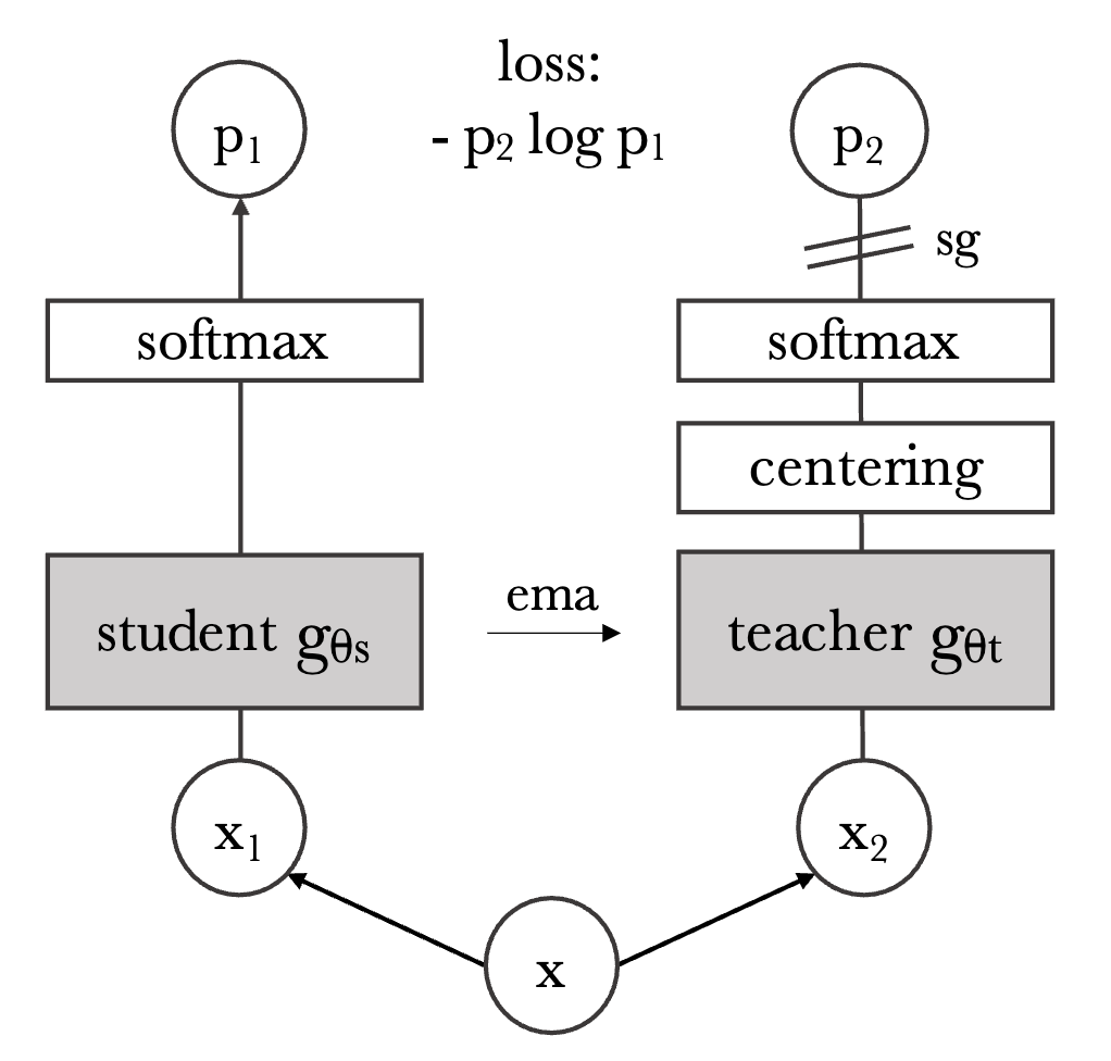
1. Two views of an image \(x\), \(x_1\) and \(x_2\) are generated through data augmentations.
   1. A multi crop strategy is used in which two large global views are generated along with a set of smaller cropped local views. The teacher only processes global views, while the student processes all views, with the constraint that the loss is not trying to match the same views to each other. This method was introduced in the SwAV paper, and helps the model learn local to global correspondences. Restricting the teacher to only global views also encourages the encoders to output global representations.
   2. Are position embeddings used?
2. The views are passed to their respective encoder (teacher/student)
3. The teacher encoding is “centered”.
   1. Perhaps centering allows this method to work without having the predictor layer. The center is a exponential moving average of the teacher encoding (of both views). This vector is subtracted from the teacher’s encoding before the softmax. A temperature is also applied with the softmax to achieve a “sharpening”. These methods help the teacher avoid collapse. Centering ensures that a single component of the vector doesn’t dominate. Sharpening ensures that it doesn’t collapse to a uniform vector.
4. Softmax is applied to each encoding. The student is trained with a cross entropy loss to match the teacher. The teachers weights are updated as an exponential moving average of the student.

This paper compares the performance of DINO with ResNet and ViT architectures against SOTA SSL methods such as BYOL, MoCov2, and SwAV. The combination os DINO and ViT has the most significant advantage. Interestingly, it is 6.6% better than ViT with BYOL training on linear ImageNet evaluation, despite minor differences in the methods. The SSL methods that are used for comparison were developed for CNN architectures, which put them at a disadvantage. DINO is designed for transformers, but what about it makes it work better with transformers? One possible explanation is that transformers handle different resolutions of images better. Higher resolution images results in more image patches generated in the transformer. The computation also scales quadratically in the attention operations with respect to the number of patches. For ResNet, the computation increases linearly.

The two main “emerging properties” they observe is that DINO ViT features are useful for dense predictions such as semantic segmentation. Another property is that k nearest neighbors on the output encodings, without any finetuning. This enables image retrieval applications.

They observe the teacher outperforms the student in DINO training. This is not observed with other SSL methods. They cite “Polyak-Ruppert averaging” as an explantation of this. This means the teacher simulates an ensemble model with its momentum weights.

The multi-crop strategy enforces that the inputs be rectangular. This makes this method compatible with CNNs in addition to ViTs. DINO shows that SSL is effective with vision transformers. However, it is designed in a way that makes the training method compatible with CNNs. This leads to some very interesting comparisons between the properties of SSL CNN and ViT models. The other works we will discuss take advantage of the flexibility of the transformer architecture, at the cost of CNN compatibility.

DINOv2: Learning Robust Visual Features without Supervision scales DINO using a 1 billion parameter ViT model along with a larger proprietary dataset. They used an interesting data processing pipeline to combine curated and uncurated data, to get a large dataset of high quality and diverse images. This step is important because unprocessed uncurated data can be of low quality and dominated by certain modes of data and duplicated data.

There are several architectural and training changes applied on top DINO v1 that allow it to scale effectively. Notably, in addition to DINO, they add an iBOT loss. This method masks some of the input tokens of the student. In order to combine DINO and iBOT losses, they learn separate heads on the student and teacher for each loss. iBOT does BERT style pretraining of image transformers, which we will also cover in this post.

data2vec

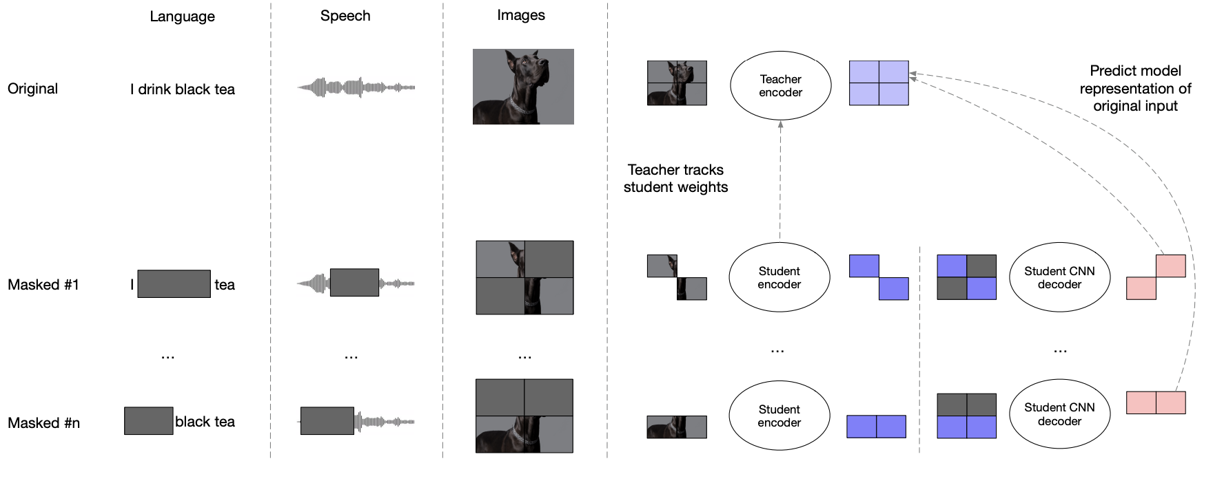
The teacher model predicts representations from unmasked input, while the student model predicts representations from masked input. The student aims to match the teacher’s output by predicting the representations of the masked tokens. To avoid collapse, the teacher’s weights are an exponential moving average of the student’s weights.

Instead of training a multimodal model, independent models are trained on different modalities. Data2VecAudio, Data2VecText, and Data2VecVision are developed. The learning objective remains the same, but the generation of embeddings and masking strategies differ.

1. Encoding of inputs into embeddings:
   1. Text is tokenized, and learned embeddings for each token are retrieved.
   2. Images are divided into 16x16 patches and linearly projected into an embedding.
   3. Audio is encoded by a 1D convolutional neural network with multiple layers. A 16 kHz waveform is mapped to a 50 Hz representation. This means a sequence of 320 integers is mapped to a single representation.
      1. Unlike images, a multiple-layer network is used for audio, likely due to the absence of a Fourier transform.
2. Masking:
   1. Some of the student input embeddings are replaced by the MASK token embedding.
      1. Text: Random tokens are masked.
      2. Images: Embeddings corresponding to rectangular blocks are masked.
      3. Audio: Continuous spans of embeddings are masked.
3. Addition of position encoding.
4. Both the teacher and student transformer models receive the input.
5. Representations at different layers are distilled from the teacher to the student. Outputs from the masked tokens of the top \(K\) transformer blocks are normalized and averaged into a single vector.
6. A regression loss (Smooth L1) is applied to the averaged vectors of each network.
   1. The loss transitions from a squared loss to an L2 loss when the error margin goes below the hyperparameter \(\beta\). The L2 loss is only applied when the student and teacher predictions are close. This loss is designed to be less sensitive to outliers.

1. The students weights are updated with SGD. The teacher’s weights are updated as a EMA of the students weights: \(\Delta \leftarrow \tau \Delta + (1-\tau)\theta\)
   1. \(\Delta\) represents the teacher’s parameters, while \(\theta\) represents the student’s parameters.

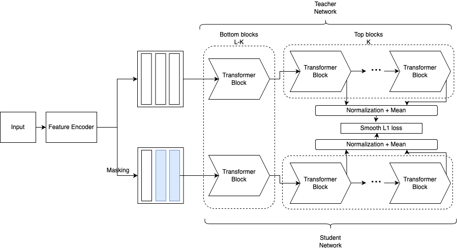
The position encoding and feature encoder weights are shared between the two models. However, the teacher’s transformer weights are specified through an exponential moving average.

data2vec 2.0

Data2Vec 2.0 introduces several architectural and loss function changes that lead to a significant speed up in training.

They use target representations for multiple masked predictions of a sample. This is more computationally efficient because we only need to run the teacher model once to train with \(M\) different masks of the input instead of 1. Further efficiency gains are implemented through not processing the masked parts of the image with the student, and sharing the feature encoder output across all masks.

They use a L2 loss instead of a smooth L1 loss. This is a simplification of the earlier loss. They also use a convolutional decoder to predict the masked representations rather than a transformer.

They also introduce inverse block masking. Rather than masking blocks. Blocks are chosen to be unmasked areas. The representations outside of the block will be predicted. There are multiple blocks which may overlap. A mask consists of multiple blocks. Training includes multiple masks for each target.

They also add a linear attention bias (ALiBi). This essentially modifies self attention to increase the bias for query key pairs that are far apart. This enables faster training by providing an inductive bias.

Masked Autoencoders Are Scalable Vision Learners

This paper uses a simple autoencoder architecture to learn image representations. Parts of the images are masked, and the model is tasked to predict what is in the masked regions. This model can be trained through this notebook.

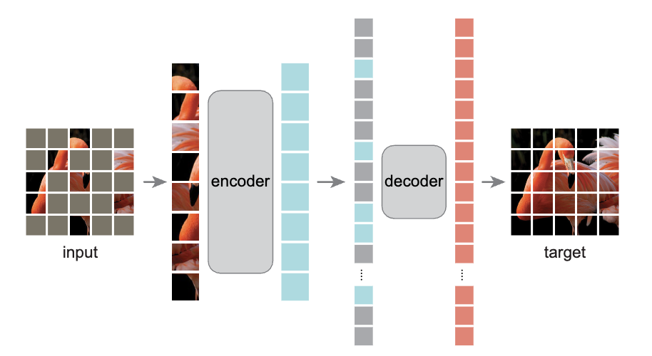
1. The image is split into patches, as done in Vision Transformers.
2. Using a mask ratio (75%–95%), patches are selected randomly without replacement.
3. The unmasked patches are input into the encoder. Note that the mask tokens do not get processed by the encoder (difference from BERT). The encoder uses a vanilla ViT architecture, where the unmasked patches are linearly projected into token embeddings which get processed by transformer blocks. The output is a ViT-processed embedding for each unmasked patch. Each patch has an added position embedding.
4. The encoded tokens and the masked tokens are combined as an input to the decoder. The mask tokens map to a learned embedding. This embedding will be the same at all positions because it is not transformed by the encoder. At this stage, position embeddings are added to the full set.
   1. Note that for unmasked tokens, position embeddings are added twice, once before the encoder and once before the decoder.
5. The decoder reconstructs the unmasked image from the set of patch embeddings. The decoder is trained by a mean squared error loss with respect to the unmasked input image.

This architecture builds on the vision transformer. An alternative is to use CNNs. This would involve directly setting pixels in the input image to zero, learning a vector representation, and then decoding it back to the image. The reason this fails is that it aims to globally decode an image. With transformers, you first predict representations of the masked patches, and then decode into the image patch. This breaks it down into two easier problems. Also, with CNNs, you can’t explicitly encode masked regions like you can with a ViT. Having a mask token more explicitly indicates the mask.

They mask a very high percentage of patches (80%). This reduces spatial redundancy and forces the model to learn more higher-level and useful features. With a lower mask ratio, the model might learn to represent small local changes, like color and lighting variation. It doesn’t need to understand the higher-level structure of the image, because it’s mostly already there. This is a notable change from language models. BERT masks 15% of tokens. MAE and related works mask a majority of the image (75%+).

The model uses the ImageNet-1K dataset for pretraining and evaluation. Evaluation is done by either finetuning the full encoder model or using a linear probe (training one MLP layer on the output of the encoder) on the task of classification.

One interesting result is that the performance of finetuning and linear probing has different trends when ablating the masking ratio. Linear probing accuracy increases linearly with masking ratio until 75%. Finetuning has relatively consistent performance between 40% and 80%.

Having a deep decoder allows for the representations to be more abstract, because the decoder has more capacity for reconstruction. A shallower decoder would lead to the encoder having to represent more of the details needed for reconstruction. This is less relevant for finetuning than it is for linear probing, as during finetuning, the encoder can shift from focusing on reconstruction to recognition. In my opinion, linear probing results are more interesting since the goal is to build useful representations that can be used for various tasks. Finetuning offers just a marginal improvement over just training on the classification task directly without pretraining at all. However, linear probing discourages learning nonlinear features in the representation. To address this, the authors evaluate “partial finetuning” in which the last few blocks of the transformer are finetuned.

Excluding mask tokens from the input and using a lightweight decoder makes this model very efficient to train. Using mask tokens in the encoder also creates a domain shift between pretraining and downstream tasks, which hurts performance. This is because a large portion of the pretraining input will be mask tokens, which is significantly different from what the model will see downstream.

BEiT: BERT Pre-Training of Image Transformers

This approach is most similar to BERT / NLP SSL models.

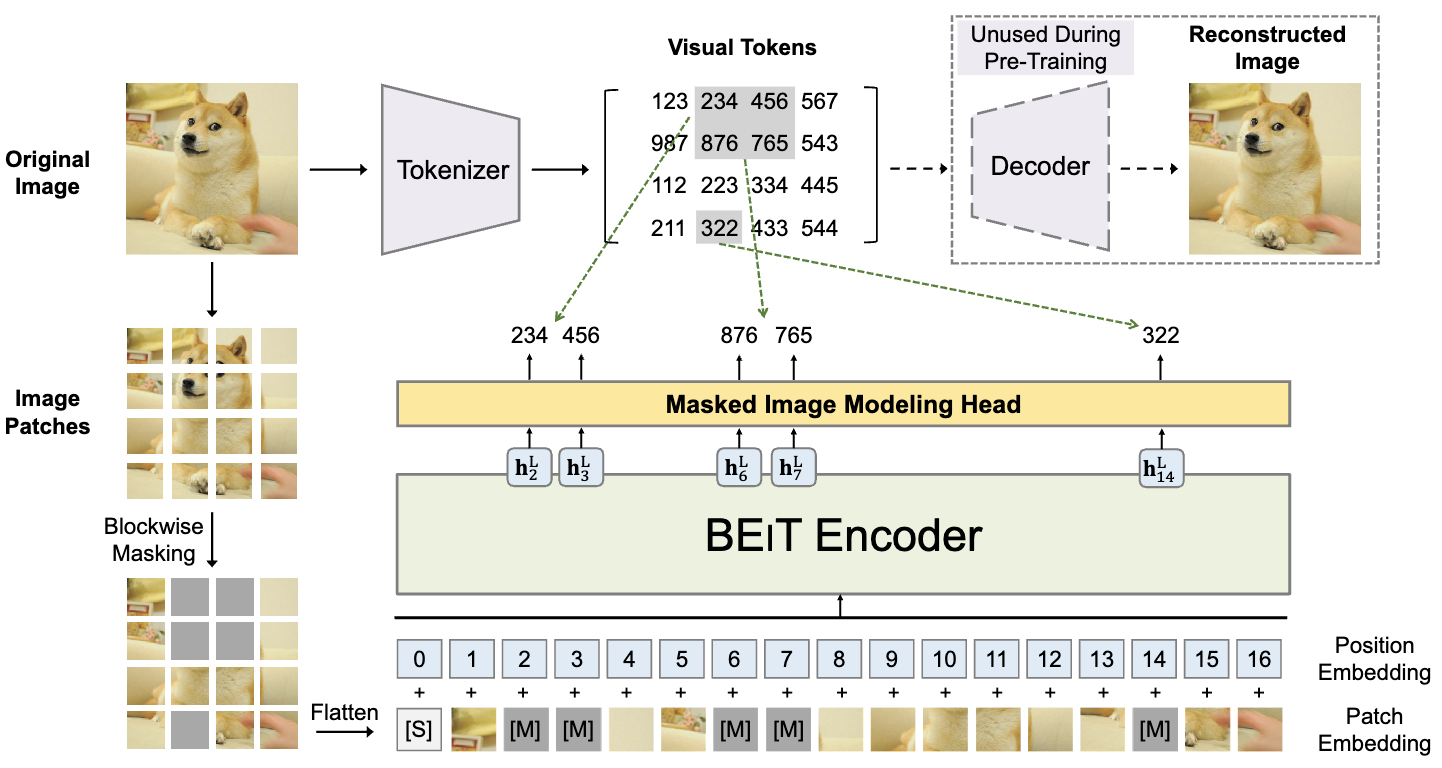
A fundamental difference in applying SSL to images compared to text is that images are continuous. Text has a finite number of tokens. You can use a softmax to get a probability distribution across all tokens. In ViTs, patches of an image are treated as tokens. However, you can’t get an explicit probability distribution over all possible image patches. BEiT addresses this problem by training a discrete variational autoencoder (dVAE) to learn discrete visual tokens. These discrete tokens are an approximation or compression of image patches.

The main difference between this and a vanilla ViT architecture is the usage of discrete visual tokens.

There are two steps to training:

1. Tokenizer and Decoder are trained as a VAE to learn discrete visual tokens
2. The discrete tokens from the learned tokenizer are used to pretrain a BEiT encoder.

Why aren’t the tokens used as the input directly? The softmax distribution of tokens could be used as a soft label for the BEiT encoder.

The transformer training task is named masked image modeling (MIM), as it is designed after BERT’s masked language modeling (MLM). 40% of the tokens are masked. Similar to other methods, BEiT masks a large portion of the image to make the pretraining task sufficiently difficult.

Conclusion

The landscape of self-supervised learning for image processing is undergoing a significant transformation. While it originated with Convolutional Neural Networks (CNNs), a strong coupling with transformer-based architectures is emerging and may lead the way for further advancements.