Many of the state-of-the-art results in deep learning are achieved using multiple GPUs. For some of the largest and most data-intensive ML models, it can take months or even years to train on one CPU or GPU. Training is sped up by scaling to large numbers of GPUs/TPUs. Some neural networks are too large to even fit on one GPU. For example, training large language models like BERT can easily exceed the available memory on a single GPU.

If you have the resources it can be easy to speed up training by adding more GPUs. However, it is important to understand the impact this scaling will have on training. Machine learning acceleration is a huge and complex field. I intend to just cover the basic intuitions to keep in mind when training a typical model.

There are two types of machine learning training parallelization: data parallelism and model parallelism.

Data Parallelism

Data parallelism splits a training batch into smaller batches for each GPU. Each GPU has its own copy of the model. Each GPU computes gradients with its own training batch. These gradients are then aggregated across all the GPUs. Each GPU can send its gradients to all other GPUs. For example, if you train with a batch size of 64 and 4 GPUs, each GPU will get a batch size of 16. It will compute gradients for this batch. Once all the GPUs are done with their computations, they can send their gradients to each other. The gradients are then averaged and applied to the model. This allows us to train a model with batch size 64 at the speed of batch size 16. However, there is additional latency in communicating the gradients and synchronizing the GPUs, but it is usually negligible compared to the gradient computations.

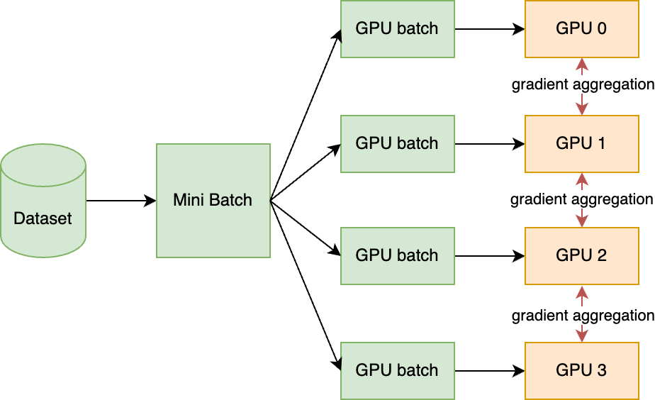
Another option is to skip the gradient aggregation and simply apply the updates to the model separately. This can be done by having an orchestrator take a lock on the model. Or in Hogwild, you can just update the model without any lock. This will allow some GPU batches to be dropped due to race conditions but minimizes synchronization delays.

Adding GPUs doesn’t make training steps faster. It allows you to have larger mini-batch sizes, which in turn trains models faster.

There are three variables to consider: mini-batch size, GPU batch size, and number of GPUs. Since the number of GPUs is a function of the other two variables, we will only discuss the two types of batch size and how to optimize them.

\[\textrm{Mini batch size} = \textrm{GPU batch size} * \textrm{Number of GPUs}\]

The implementation of parallelism can vary between ML frameworks: PyTorch, TensorFlow, Jax

Optimal GPU Batch Size

With GPUs, we simply want to minimize the training step time. If we operate the GPUs in the optimal GPU batch size range, we can then just set the number of GPUs to get the optimal mini-batch size. Also, note the GPU batch size has an upper limit from the memory available.

To see how GPU performance relates to speed, I timed the training steps of a ResNet50 model against ImageNet-sized batches of different sizes. I tested batch sizes of every power of two until the GPU ran out of memory.

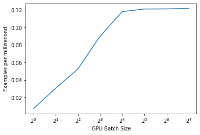
We see that the throughput (examples per ms) is maximized at the largest possible batch size. We also see that for batch sizes of less than 2^4 or 16, the throughput is lower. GPUs are inefficient with small batches due to overhead. CPUs perform better in some settings. The takeaway is that we want to maximize the GPU utilization by fitting the largest possible batch. Some libraries have the functionality to search for the largest possible batch size given a GPU and dataset. In the flat region, GPU step time increases linearly with batch size.

Optimal Mini Batch Size

To optimize the mini-batch size, we will ignore accelerators and just focus on mini-batch gradient descent. Mini batch size is less hardware-dependent and more problem dependent. We will use ImageNet as an example, but the effects of batch size on training should be considered for every new problem.

Assuming maximize GPU usage/batch size, optimizing the mini-batch size means selecting the number of GPUs to use. The assumption is that with more GPUs, we can train a model faster. Training on more GPUs means faster training epochs. However, we are interested in the test accuracy of the model, not just completing epochs.

Consider this plot from the paper Measuring the Effects of Data Parallelism on Neural Network Training by Shallue et al.

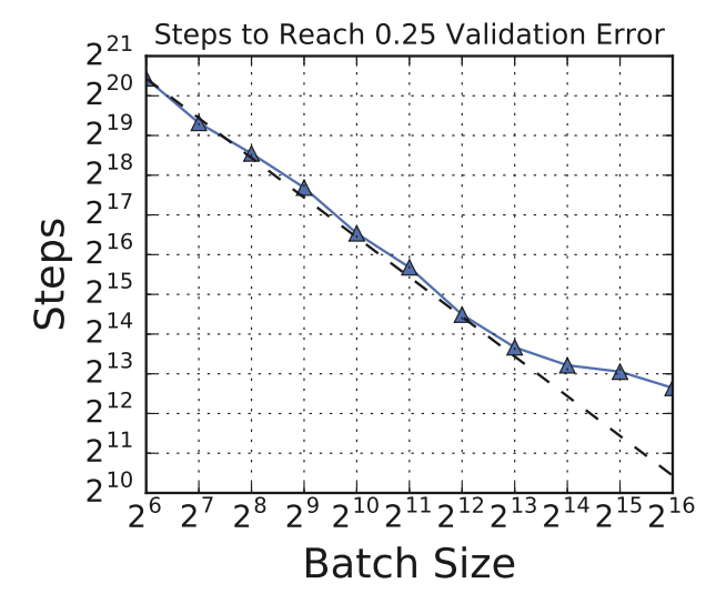
For points on the dashed line, the number of training steps is halved whenever the batch size is doubled. This means that doubling the GPUs/TPUs would have the training time. This is ideal. In this region, you can happily speed up your model training by adding more GPUs that you may have available. However, this tradeoff changes at batch size 2^13 or 8192. From here, doubling the GPUs still speeds up model training, but the speed will be more than half. This is the point of diminishing returns. If you have the GPUs, you might as well use them but those additional GPUs are not as effective.

The paper goes into great detail on this relationship and the effects of other factors such as model architecture, optimizers, and datasets. The takeaway for this blog is that if you set the maximum GPU batch size, up to a point, adding additional GPUs will linearly speed up the training of your model.

Model Parallelism

This type of parallelism is much less commonly used. It can be used along with data parallelism. Model parallelism is when an ML model is too large to fit in the memory of one device. It is partitioned across multiple devices. This has enabled us to train larger and larger networks. For example, the GPT-3 model is about 350 GB. No single GPU can store the whole model in memory.

There are different ways of achieving model parallelism. You can split the model vertically by layer, or horizontally by splitting the tensors.

Pipeline Parallelism

The simplest solution is to process different layers of a neural network on different accelerations. A simple illustration of this:

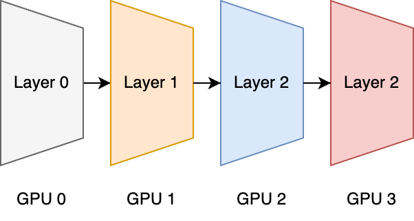
In PyTorch, the layers are bucketed into groups of roughly equal memory so that the computations are evenly distributed across the accelerators.

A major issue with this approach is that after Layer 0 has a forward pass, it has to wait for the other layers to compute forward and backward passes. The GPU is idle for about 75% of the time. The following diagrams are from the GPipe paper by Huang et al.

The solution is to have the layer compute the next graph while it is waiting for the gradient of the current batch. This essentially combines data parallelism with model parallelism. I explained above that to maximize training speed, we want to maximize the utilization of accelerators. For large models that require model parallelism, we have an additional problem of GPU waiting time. Pipelining GPU batches helps reduce this gap.

We see that with 4 GPU batches, each GPU is idle for about 6/16 of the time. The variables here are the number of GPUs and number of GPU batches per GPU. With 1 GPU batch (no pipelining), the utilization is: \(\frac{2}{n_{GPU}* 2} = \frac{1}{n_{GPU}}\). With pipelining, we get \(\frac{n_{batches}*2}{n_{batches}*2 + 2* (n_{GPU}-1)}\). This simplifies to the following:

\[utilization = \frac{n_{batches}}{n_{batches} + n_{GPU}-1}\]

This equation explains the tradeoff. Increasing the number of GPU batches drives the utilization closer to 1, while increasing the number of GPUs reduces the utilization.

In an optimal setup, we split the model among as few GPUs as possible, but increase the number of batches that they process in a step. Pipeline parallelism has the added benefit of the speedups of data parallelism. This makes it a very effective solution.

In the PipeDream paper, Harlap et al. show that we can further reduce idle time by interleaving forward and backward operations.

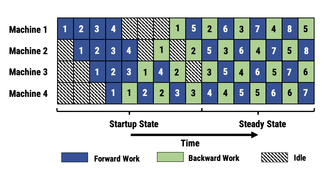
However, this eliminates gradient synchronization. Even eliminating batches above 4, we get the same utilization as GPipe parallelism, just in a different order. For many of the backward passes, a stale version of the model parameters is used. Gradient synchronization is an important tradeoff in all types of ML parallelism.

In analyzing utilization, we have been assuming that forward and backward computations are equivalent. Backward passes tend to take more time. If we interleave operations as to always prioritize backward passes, we can get a utilization gain. From AWS Sagemaker documentation:

The idle time here is 1 forward pass and 1 backward pass.

With backward prioritization, the idle time for GPU 0 is 3 forward passes. This effect will be increased with more GPUs. There are many tradeoffs in parallel ML, such as communication between model layers, the memory overhead of forward and backward passes, different model splits, staleness, etc. We are only covering the high-level intuitions to achieve fast and effective training of large models.

What if we want to use more GPUs for data parallelism, but without splitting up the model further? We can simply run pipelines in parallel. For example, we can split the model among four GPUs but duplicate each model split twice. We can then aggregate the gradients of both pipelines in the update. This is often called hybrid model and data parallelism.

Tensor Parallelism

Instead of splitting the model into layers, we can split the layers themselves. From the Megatron-LM paper by Shoeybi et al.:

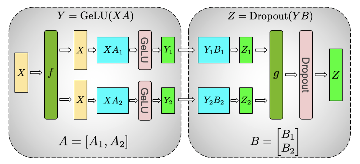
The input X has to be completely copied for each split of the model. The layer is split into two halves. The splits of the model are then aggregated in the last layers of the model. Splitting the tensors themselves offers some benefits. The latency is reduced since you can fit more layers on a GPU. This is parallel computation instead of serialized computation. You don’t have to worry about scheduling to minimize idle time.

An issue with this approach is that the activations are also separated, so you are learning a different model architecture. There is an additional cost in concatenating \(Y_1\) and \(Y_2\) for both GPUs. The Megatron-LM architecture is designed to reduce the cost of communicating between GPUs.

Conclusion

We touched the surface on the many tradeoffs, optimizations, and considerations needed for distributed and large scale ML. As models grow larger, it will become more import to understand and keep up to date with this field.

Additional Resources

https://www.youtube.com/watch?v=3XUG7cjte2U

https://lilianweng.github.io/posts/2021-09-25-train-large/

https://openai.com/blog/techniques-for-training-large-neural-networks/

https://timdettmers.com/2014/10/09/deep-learning-data-parallelism/

https://huggingface.co/docs/transformers/v4.15.0/parallelism