Yann LeCun describes self-supervised learning as the next big challenge in the field of AI. How does it work? Self-supervised learning (SSL) is a specific type of unsupervised learning. It aims to learn from large datasets of unlabeled data to enable building more robust models in different domains such as vision and NLP.

For many computer vision problems, it is a common practice to pretrain the model on a supervised learning task. For example, there are many neural networks that are pretrained to do image classification on ImageNet. However, self-supervised learning has recently been shown to outperform supervised pretraining learning on certain tasks. SSL is an active area of research with heavy involvement from top AI labs in Google, Facebook, Deepmind, and academia. Rather than focusing on the details of SSL architectures, we will explore the intuitions on why it works and what is needed.

Code

In order to make it easy to directly interact with SSL, I wrote a Colab notebook showing a few algorithms. This notebook demonstrates transfer learning on CPC, SwAV, and SimCLR pretrained models on the CIFAR10 classification task. This uses PyTorch Lightning’s implementations of these algorithms.

We are experimenting with the simple example of pretraining on ImageNet and evaluating on CIFAR10 classification. SSL can be effective on other datasets and learning tasks (object detection, segmentation, etc.), but these won’t be the focus of this post.

Motivations

Data

Self-supervised learning does not need labels. The amount of unlabeled data generally far exceeds the amount of labeled data. SSL can leverage large amounts of unlabeled data to build powerful models. Although most research does not use datasets larger than ImageNet, there are real world applications of using larger unlabeled datasets. For example, Facebook/Meta can train the SEER model on billions of Instagram images.

Generalizability

If you train a model on image classification, it may not perform as well on non-classification tasks. This is because only part of the image’s information is needed to classify it. A self-supervised learning algorithm may be able to use more of the information in the data.

The reason for the generalization gap is that the classification task does not always require a strong understanding of the object. For example, if you trained a supervised model to classify dog breeds, it may only look at the texture and color of the dog’s fur. In order to classify the breeds, the network may not need to understand other characteristics of the dog, such as size and facial features. This model would then not generalize well if you want to add a new dog breed with an indistinctive skin pattern. It will also not generalize well to new tasks like classifying the size or shape of the dog.

Better Performance

It is common to think that unsupervised / self-supervised learning is only useful when you lack labels to do supervised learning. However, these approaches can actually increase performance compared to a fully supervised approach. The ability to learn more accurate and robust models is what gives self-supervised learning the potential to shift the field of AI.

In research, there are comparisons between training on ImageNet images and labels with supervised learning and ImageNet with only images for self-supervised learning. Although the motivation for SSL is often framed as being able to use more data, in this case, the size of the dataset is the same. The ability to use larger unlabeled datasets is just a side benefit of SSL.

Vision vs NLP

Self-supervised learning has been long applied in NLP, but as Yann LeCun and Ishan Misra point out, it is much harder to apply to vision. In NLP, language models are often trained with self supervision. Given a some text, you can mask a word and try to predict it given the rest of the text. There is a limited vocabulary, so you can assign a probability to each word. This is the basis of many popular NLP methods.

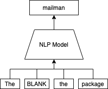
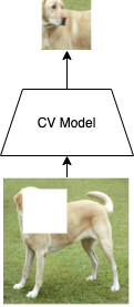
The analogue for vision is to mask a patch of an image and try to fill it in. However, because there is an intractable number of possible ways to fill in an image, you can’t compute a probability for each one. There can also be a large number of possible solutions. For example, in the image above, there is many facial expressions the dog could have. The NLP approach is straight forward but cannot be directly applied to vision.

Pretext Task

The earlier approaches to self-supervised learning focused on training the network on a pretext task. This task would not require labels in the label. The labels will be made up through the task. In RotNet, each image is rotated by 0, 90, 180, or 270 degrees, and a network is trained to predict the rotation. In Jigsaw, the image is split up into patches and scrambled like a jigsaw puzzle. A network is then trained to solve the puzzle by predicting the permutation.

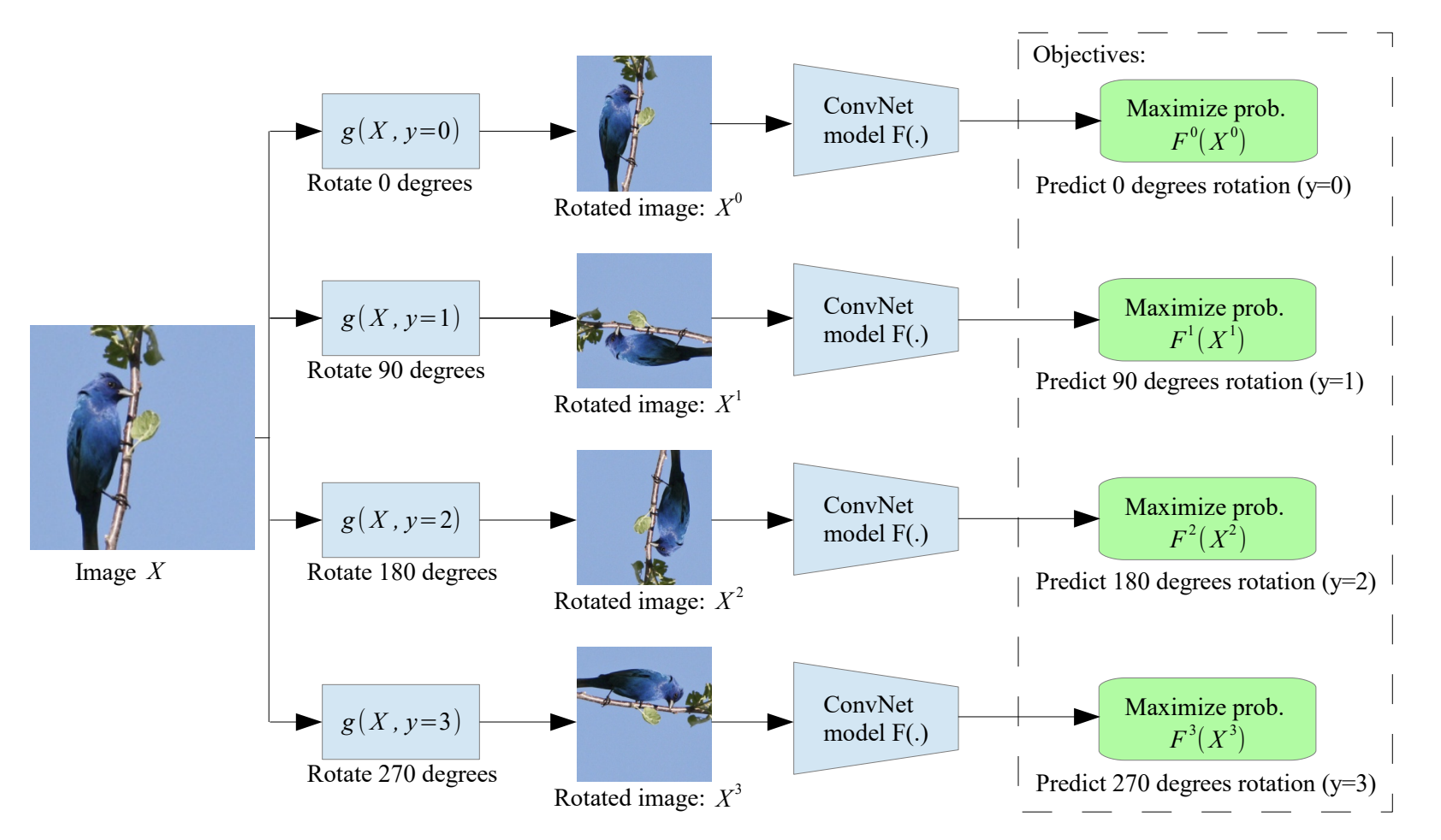
The problem with pretext task-based SSL is the same as supervised learning. There can be shortcuts to achieve high accuracy on the task. There have been attempts to avoid this. For example, in Jigsaw, each path is randomly cropped, so the task can’t be solved by simply lining up edges. However, the limitations still exist regardless, so more recent research has focused on contrastive learning.

Contrastive Learning

A neural network outputs a vector representation for every image. The goal of contrastive learning is to push these vectors closer for similar images and pull them apart unrelated images. This in different ways in different research papers.

CPC

Contrastive Predictive Coding is a method developed by Deepmind. It is a generic approach that can be applied to any data modality. In the paper, it is applied to images, audio, and text. It is a very general framework with two main components: an encoder, and an autoregressive model. These can be anything and are designed to fit the domain.

The encoder simply encodes the data into a lower-dimensional vector \(z_t\). This can be any model. For images, this can be a convolutional neural network.

Autoregressive models the variables in the data are given an order. In images, the pixels can be ordered from left to right and top to bottom. We can imagine unrolling each datapoint (ex: image, audio clip) into a list. We can call each element of this list an observation. CPC encodes a sequence of observations \(X\) into a sequence of encodings \(Z\).

\[X = [x_1, x_2, x_3, x_4 ... x_N]\\ Z = [z_1, z_2, z_3, z_4 ... z_N]\\ z_t = g_{enc}(x_t)\]

The prediction of an observation in the sequence depends only on the previous observations. This similar to predicting the future from the past in a time series. In CPC, the autoregressive model is used to generate context vectors from the encodings \(z_t\). Context vector \(c_t\) is a function of encodings \(z_{\leq t}\), but not any encoding after \(z_t\). Note that the autoregressive model is trying to predict the encodings of the observations, but not the observations themselves. The architecture of this autoregressive model depends on the application.

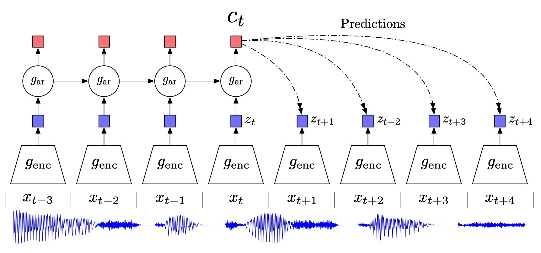
With these two models, we can generate an encoding of the data and context vectors. These vectors can be used as representations of the data. But how are these models trained? The self-supervised task is essentially predicting the input from the context. For example, given \(c_t\), we want to be able to go backwards and identify that it was generated from \(x_t/z_t\). The models are trained on a contrastive InfoNCE loss.

\[\begin{equation} \mathcal{L}_{\mathrm{InfoNCE}} = -\mathbb{E} \left[ \mathrm{log} \frac{ s(x, y) } { \sum_{y_j} s(x,y_j) } \right] \end{equation}\]

\(x\) is the sample we are trying to predict. \(c\) is the correct context. \(c_j\) are the context vectors for the negative samples. The negative samples come from other observations of the same datapoint and other datapoints in the batch. We want to maximize \(s(x,c)\) and minimize the sum of \(s(x, y_j)\). This is contrastive in that we are pushing \(y\) to be close to \(x\), and all other \(y_j\) to be far from \(x\).

\[\begin{equation} f_k(x_{t+k},c_t) = \mathrm{exp} \left( (g_{enc}(x_{t+k}))^TW_kc_t \right) = \mathrm{exp} \left( z_{t+k}^TW_kc_t \right) \end{equation}\]

The \(s\) function is modeled by \(f_k\) a log bilinear model. \(W_k\) is linear transforms the context vector, which can then be compared with the encoding \(z\).

To apply this to vision, the image is split up into 7x7 patches (with 50% overlap) which will be considered the observations. Each patch is encoded by a CNN (ResNet without pretraining). If the encoding returns at 1024 dimensional vector, the encoded image will have a size of 7x7x1024. An autoregressive model (PixelCNN or PixelRNN) is applied to the encodings of the patches. For 1D data like audio, an RNN/LSTM scan be used. The self-supervised task in this case is predicting which patch generated each context vector. Refer to the PixelRNN paper for more information on autoregressive models and PixelCNN. The final representation is computed by mean pooling the encodings into a single 1024 dimensional vector. This can then be used for downstream tasks, like image classification.

Why do we need the autoregressive model? We could optimize the InfoNCE loss using the 7x7 encodings. The self supervised task here is predicting the next context vector given a sequence of context vectors. This is similar to predicting the next patch of an image given all the previous patches. But rather predict the patch, which as we discussed is too difficult, we just predict a lower dimensional vector. Without this autoregressive constraint, we are just optimizing for generating unique embeddings for each patch and ignoring the relation between the patches. The InfoNCE loss is just ensuring that the predictions are correct.

Why not just mask out the current context / observation? The architecture for this may be a masked fully connected layer that learns the context vector for each observation, while excluding the connection to the observation itself. Or there could be two PixelCNNs, one from the left and one from the right. We can then concatenate these two context vectors and possibly add additional neural network layers on top of it. Both methods would be more computationally expensive and complex, but likely still feasible. This would be bidirectional model for images similar to BERT. This idea may be explored in other research papers or, it may be an open idea to try.

SimCLR

SimCLR is a method from Google Brain which takes a different approach for self-supervised learning of image representations. The basis of SimCLR is image augmentations. Image augmentation has long been used in supervised learning. The augmentations are transformations applied to the image and cropping, color change, and rotation. The idea is that these transformations do not change the content of the image and the network will learn to ignore and be invariant to these transformations. In supervised learning, data augmentation is used to just increase the size of the dataset for a supervised task like classification. Many SSL methods including SimCLR make invariance to the augmentation the actual learning objective. The augmented images are fed into an encoder to get the representation. These representations are then learned to be close of augmentations of the same image.

However, the problem with just comparing within the same image is collapse. The network would learn the trivial solution of a constant vector for all representations (ex: a vector of all zeros). This would maximize the similarity between augmentations but obviously not contain any useful images. We need negative samples to minimize similarity with. In SimCLR, the negative samples are augmentations of other images from the same training batch. The assumption made here is that the other images are unrelated to the current image and the representations should be far apart.

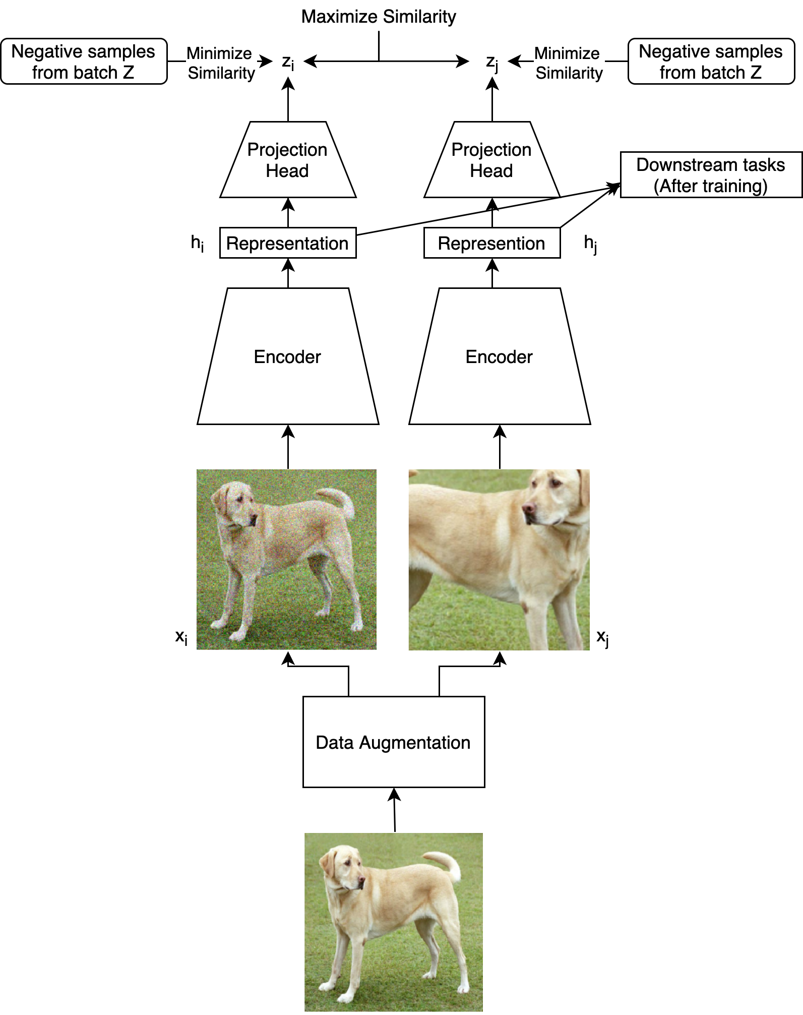
Why do we need a projection head? It would not change the architecture much by optimizing the similarity losses on the representations themselves. The encoder may even include the same fully connected layers that would have been in the projection head. The projection head allows for a more complex and nonlinear similarity relationship between the encodings. Without it, the representations would have to have a high cosine similarity. This may restrict the expressivity of the vectors. The projection head can also ignore some information in the representations. For example, SimCLR may train to make the representations invariant to rotations. The rotation angle may be encoded in the representation but ignored by the projection head. If the rotation is encoded in the first 5 values of the vector, the projection MLP may have zero weights for those values. This may be desirable in a variant of the architecture in which the self-supervised learning happens simultaneously with a downstream task. The SimCLR architecture itself has no reason to include unnecessary information in the representation. It is unclear whether having “extra” information in the representation is desirable or not.

Projection heads are very common in self-supervised learning. The autoregressive model in CPC can be viewed as a projection head.

Aggressive augmentation yields the best results. This means applying multiple augmentations at a time. This makes the contrastive learning more challenging and forces the network to learn more about the image. The augmentations also avoid trivial solution to the contrastive objective. Without cropping, the network can match two augmented images by their local features (edges in the same place), instead of learning global features. Without color distortion, images can be matched by their color distribution. These augmentations can be composed with others, such as rotation and blur.

\[\begin{equation} \ell_{i,j} = \log{\frac{\exp(\mathrm{sim}(z_i,z_j)/\tau))}{\sum_{k=1}^{2N}\mathbb{1}_{[k\neq i]}\exp(\mathrm{sim}(z_i,z_k)/\tau)}} \end{equation}\]

The loss is referred to as NT-Xent (the normalized temperature-scaled cross entropy loss). The similarity function \(s\) can simply be cosine similarity (\(\frac{u^\top v}{\|u\|\|v\|}\)). This loss is similar to the InfoNCE loss. The main difference is the temperature \(\tau\). The temperature essentially controls how strongly should attract and repel the other vectors in the loss.

Scaling

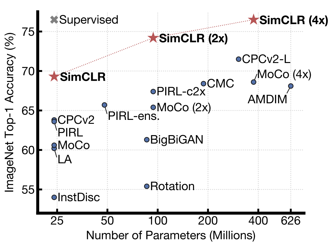
Self-supervised learning is often evaluated on ImageNet classification. The projection head is replaced with a linear layer. The network is then trained to classify ImageNet with the encoder weights frozen. The encodings learned with self-supervision must be useful enough for a linear layer to classify them.

An interesting property of self-supervised trained encoders, is how the scale in terms of depth and width. We see that only SimCLR(4x) is able to match the accuracy of fully supervised learning. “4x” means the network is 4 times as wide and as deep. It is not necessarily a bad thing that SSL requires a much larger network for ImageNet classification. This likely means the network is learning more information from the data than what is needed for supervised learning. Although this doesn’t help with ImageNet classification, the vectors may be more effective in other downstream tasks.

One issue with SimCLR is its reliance on huge batch sizes. The best results come from a batch size of 4096. It needs many negative samples to be effective. This makes the network inefficient to train. Other approaches attempt to address this problem.

BYOL

BYOL is a paper from Deepmind that aims to remove the need for negative samples. There are two networks: a target network and an online network. The target network’s weights are an exponential moving average of the online encoder. Similar to SimCLR, augmented versions of an image are passed through the encoders. Unlike SimCLR, the loss does not use negative examples so there is no need for large batch sizes. There is a projection head on top of the online encoder. The online encoder is used for downstream tasks.

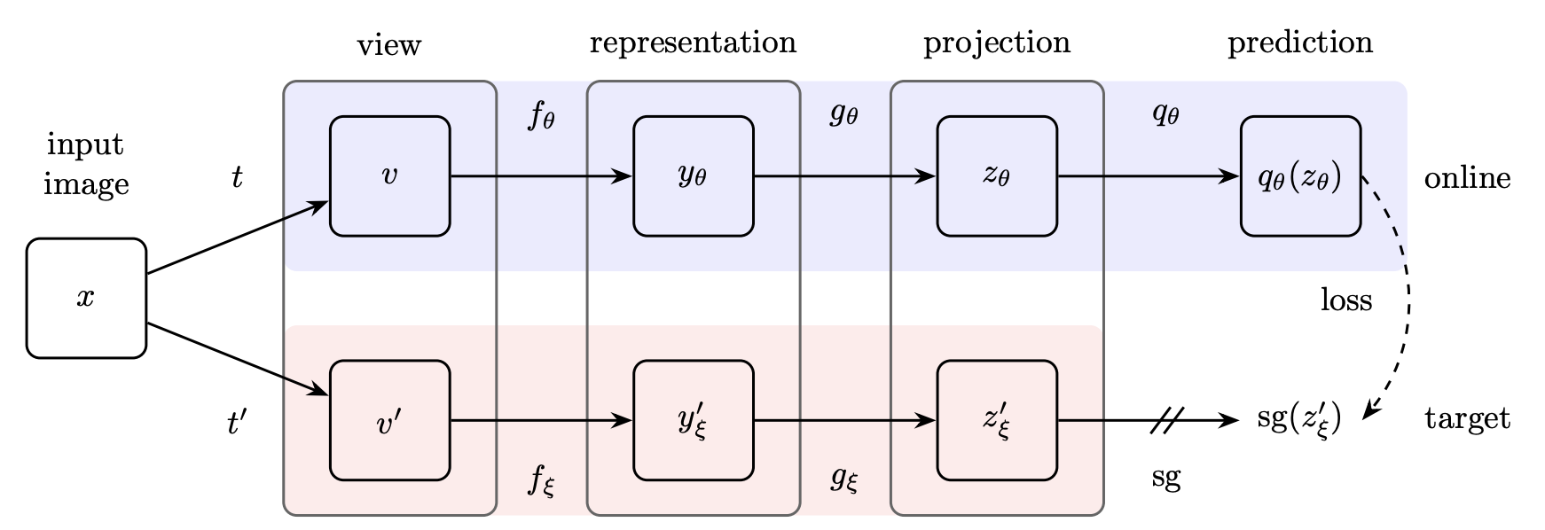
Bootstrapping is a poorly defined word used in machine learning. It can mean simultaneously optimizing two objectives that depend on each. In BYOL, that refers to the two encoders.

BYOL is able to learn useful representations without collapse because only the parameters of the online encoder are optimized. The online encoder can’t learn to output a constant because it is following the representations of the target encoder. The bootstrapping ensures that the trivial solution is avoided.

BYOL is a non-contrastive method of SSL. However one criticism of BYOL is that batch normalization causes implicit contrastive learning by leaking information between batch elements. However, in a follow up paper, the authors show that replacing batch normalization with group normalization and weight standardization leads to comparable performance.

Clustering

Clustering is an important class of unsupervised learning algorithms. Although more often used outside of deep learning, clustering can be applied to self supervised learning. Feature vectors can be clustered. Clusters can indicate a group of related images. In this sense clusters are similar to classes and can be used as labels in SSL.

DeepCluster

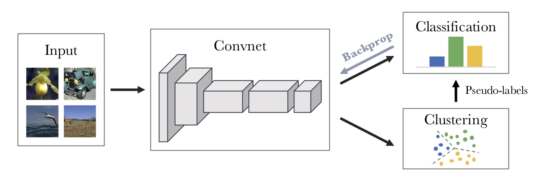
DeepCluster trains a neural network in two alternating steps: clustering and classification. In the clustering step, each image is assigned a cluster as a pseudolabel by clustering the feature vectors from the network. K-means is used for clustering. There are \(k\) clusters of the same dimension as the feature vectors. The network is then trained to predict the clusters from the images. After training on this classification objective, the features improve. The dataset is reclustered with better clusters. This iterative training procedure improves the clusters and the representations.

The main problem with DeepCluster is that it requires periodically clustering the entire dataset. This limits this method in scaling to extremely large datasets. This is addressed by SwAV with an online approach to clustering based SSL.

SwAV

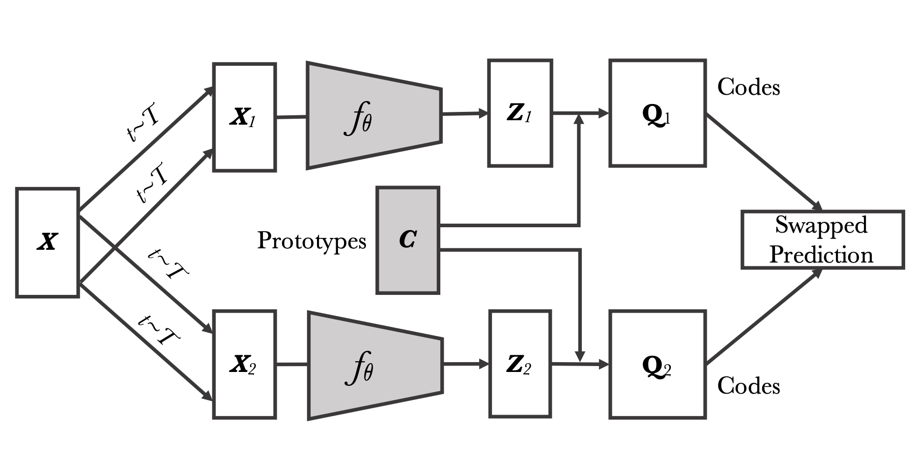
SwAV extends on DeepCluster to be online, while also taking inspiration from contrastive SSL methods. Two augmentations of an image are passed to an encoder. These representations are then assigned prototypes. There are K prototypes, which are vectors of the same representation as the encoding.

Conclusion

There are many approaches to self supervised learning, however there are common elements. There are contrastive losses, data augmentation, bootstrapping, projection heads, and sometimes negative samples.