The Transformer architecture has emerged as the cornerstone of deep learning and artificial intelligence. Despite its conceptual simplicity, the specific details of the architecture can be difficult to understand and reason about. This two-part blog series aims to provide a thorough examination of the Transformer, demystifying its core components and recent advancements. The goal is to cover the fundamental and cutting-edge concepts needed to design transformer-based models for any application in any modality.

This blog post will be in two parts:

Part 1 will be a deep dive of the standard Transformer architecture. It is a highly modular architecture, so we will explain each component in detail and how they integrate. This will also cover how to design the components for different use cases. It was introduced by the famous paper Attention Is All You Need. There is no shortage of resources to learn about transformers, but I hope to offer some new perspectives.

Part 2 will cover recent advancements that have further advanced the capabilities of transformers. The original transformer architecture is robust and versatile and has led to many successful applications. However, in recent years with the surge in investment into transformers / LLMs, we have seen many useful advances. These impart new capabilities such as longer context length, faster training, and more efficient inference. This is a guide to designing modern transformer architectures for any use case.

Transformer Architecture

Attention Is All You Need introduced the transformer architecture in 2017 specifically for machine translation. Since then, architectures derived from this have been used not only for various NLP tasks but also for other modalities such as vision, audio, and time series. We’ll take a modality-agnostic approach. As we explore each component, we’ll focus on how to design it for different modalities and use cases. For instance, position embeddings might be designed differently for text than for images.

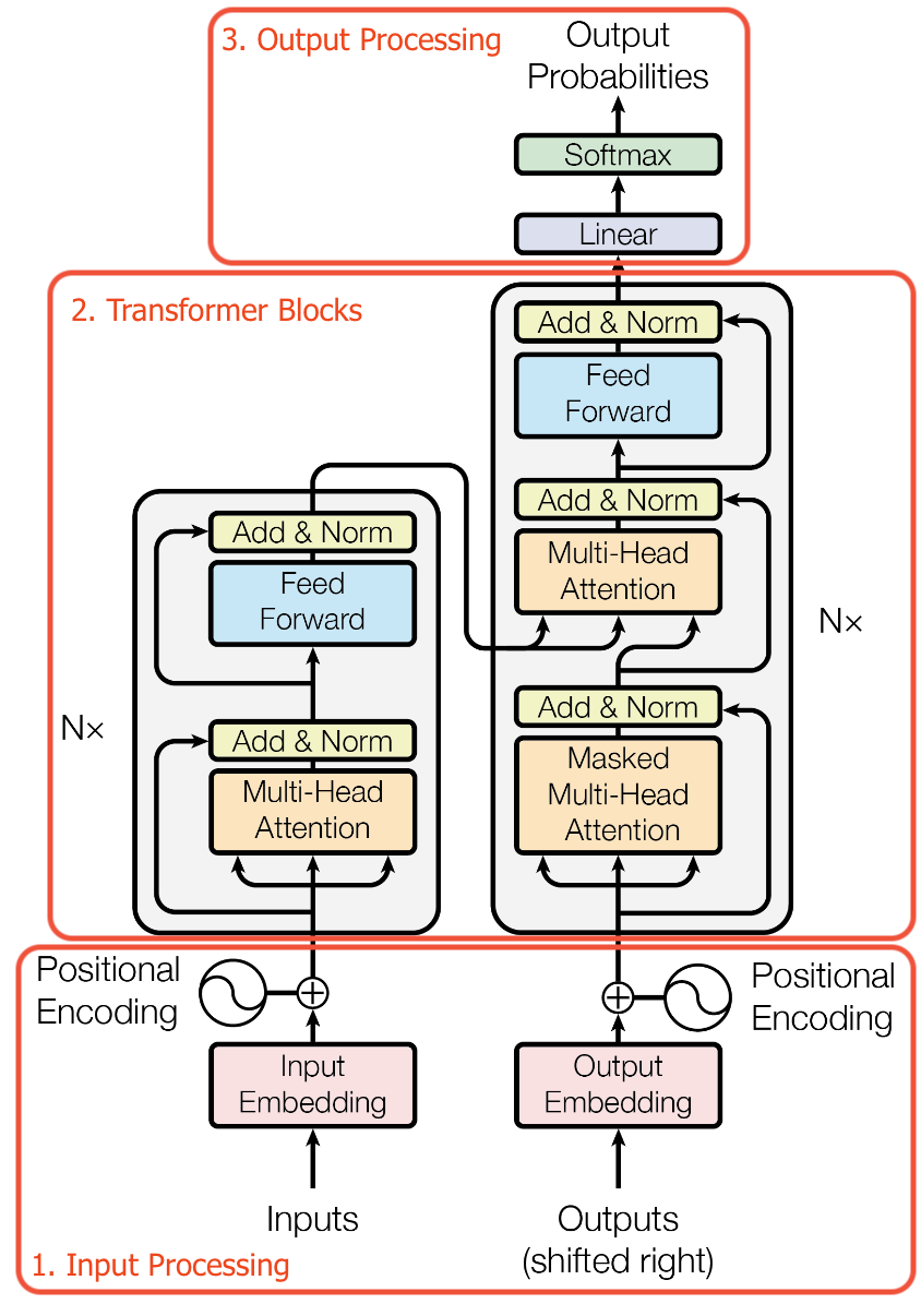
Transformers are so generalizable because they have relatively few inductive biases. Unlike CNNs, which require Euclidean input, Transformers do not enforce a data structure. It is up to the designer to incorporate domain-specific inductive biases into the model. These design decisions are important for the model to be effective at a given task.

---

The transformer architecture can be understood as 3 steps.

1. Input processing (Generation of a set of embeddings to input into the transformer)
2. Transformer blocks (Bulk of the computation)
3. Output processing (Using the output embeddings of the transformer to perform a task and train the model)

Input Processing

The input to the transformer is an unordered set of embeddings. These embeddings are high dimension vectors of floating point values that represent a part of the input. We refer to input processing as the steps taken to compute these embeddings. Input processing changes the most between modalities.

The general pattern for input processing is as follows

1. Split up the input into pieces
2. Map each piece to an embedding

The output of these two steps is a set of embeddings that represent the raw input in a way the transformer architecture can process.

Image Processing

Transformers for images were introduced in the ViT paper. The input image is processed in two steps:

1. The image is split into patches of 16x16.
2. The pixel values of each patch are flattened to vector and fed through a learned linear projection, resulting in patch embeddings.

The result is a set of embeddings that can be processed by the transformer.

Text Tokenizer

Text is represented as a sequence of characters or bytes. Unlike images, text isn’t inherently numerical data that can be directly transformed into embeddings. Text is processed by tokenization, which is mapping it to a sequence of discrete tokens. Tokenizers create a vocabulary, which is mapping of all possible tokens to vocab indices. These indices are used to retrieve a learned embedding from a table. Text input processing involves two steps: tokenization and embedding lookup.

Let’s consider two basic options for tokenization:

• Character-Level Tokenization: Every character in the text becomes a separate token. This creates a very long sequence but has a very small vocabulary.
• Word-Level Tokenization: Each word is a distinct token. This results in a more manageable sequence length but results in a huge vocabulary.

There is an obvious tradeoff between vocabulary size and input size. Character-level tokenization creates very long sequences, which can be inefficient for transformers. On the other hand, word-level tokenization can lead to a massive vocabulary size, requiring a large embedding table. This can be computationally expensive and struggle with unseen words or typos.

The ideal approach considers several factors:

• Sequence Length: Shorter sequences are generally more efficient for processing, but extremely short sequences may not capture enough context.
• Embedding Table Size: A larger vocabulary requires a bigger embedding table, increasing memory usage and training time.
• Rare Words: Very infrequent tokens may not be adequately learned during training, impacting model performance.
• Token Complexity: A single token shouldn’t represent too much information. Complex concepts might benefit from being broken down into smaller tokens for better processing by the model.

In practice, finding the right balance often involves a compromise between character-level and word-level tokenization. Techniques like subword tokenization (splitting words into smaller meaningful units) can offer a middle ground, achieving a balance between sequence length, vocabulary size, and capturing text information effectively.

Byte Pair Encoding (BPE)

The most common approach to implementing sub-word tokenization is Byte Pair Encoding (BPE).

It works by first starting with the individual characters (bytes) in the text as its initial vocabulary. This ensures that all text can be encoded, though not efficiently. BPE then iteratively identifies the most frequently occurring pair of characters and merges them into a single new token. This process continues until a predefined maximum number of tokens is reached, preventing the vocabulary from becoming too large.

One interesting feature of this approach is that the tokenizer uses a small and separate dataset for BPE. This dataset can be engineered to achieve certain properties in the tokenizer. For example, it is beneficial for this data to be balanced between different languages. For example, if the amount of data for Japanese is significantly lower than that for English. Rare pairs in English would be prioritized over common pairs in Japanese. This would be unfair to Japanese, and Japanese text would require far more tokens. To address this, the tokenizer dataset can be balanced between different languages.

See platform.openai.com/tokenizer for an interactive demo on how text is tokenized and mapped in token indices.

BPE also involves some hardcoded rules. Some bytes, such as punctuation can be ignored in the tokenizer merging. GPT tokenizers use different regex patterns to split the string prior to tokenization to prevent certain bytes from merging.

BPE is expensive to run and to encode/decode text since it is an iterative process. This is optimized by OpenAI (tiktoken) by implementing it in Rust. SentencePiece by Google is another popular tokenizer. SentencePiece runs BPE on Unicode code points (Unicode characters). It falls back to bytes for rare code points. Unicode has nearly 150k code points, a large number of which are very rare. Most tokenizers use less than 100k tokens. Having 150k tokens before adding more through BPE is not practical.

Once we have a trained tokenizer, we use it to map input text to token indices. These token indices are mapped to learned embeddings. Transformer models often include embedding tables, which store learned embeddings for each item in the model’s vocabulary.

See this video by Andrej Karpathy for a deep dive into text tokenizers.

Audio and Other Modalities

Like images, audio is a continuous data modality. A popular method of tokenizing audio is to generate a spectrogram using a Fourier Transform. This creates an image that can be tokenized in the same way as images in ViT. The AST: Audio Spectrogram Transformer paper does exactly this.

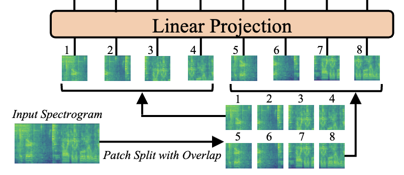
This paper uses a 2D position embedding so they can warmstart from a ViT model. If it were to train from audio only, a 1D position embedding could be used, as in OpenAI’s Whisper.

We have covered the basic methods for tokenizing text and continuous data domains, however, there is a lot of research covering alternative methods. This includes vector quantization which generates discrete tokens from continuous data modalities.

Position Embedding

The transformer takes a set of tokens as input. However, many inputs are better represented as sequences, such as text and audio Where a token occurs in the sequence is a crucial piece of information. Position embeddings can be added to the token embeddings to encode the position of the token in the sequence. Although the input is still a set, we are not losing the information of the order of the tokens within the input sequence. Position embeddings implicitly turn the transformer from a set processing architecture to a sequence processing one.

The original transformer paper evaluates two methods of configuring the position embedding. These have equivalent results.

• Learned: A separate learned embedding is used for every position in the sequence up to the maximum sequence length.
• Fixed: The embedding values aren’t learned but are configured as a function of the position. \(i\) is the index in the embedding. \(d_{model}\) values have to be generated so the position embedding can be the same dimension as the token embedding.

\[PE_{(pos,2i)} = \sin\left(pos/10000^{2i/d_{model}}\right) \\ PE_{(pos,2i+1)} = \cos\left(pos/10000^{2i/d_{model}}\right)\]

These embeddings are added to the input token embeddings. This assumes that the addition of the positional encoding doesn’t cause conflicts in the embedding space (which is typically in a high dimension). However, it is also possible to concatenate position embedding values.

For language, 1D position encodings are used. These embeddings should be designed to fit the data. For example, in images, the position embedding is 2 dimensional. For videos, an additional time dimension can be added. The embedding can be designed in any way to encode the structure of the data.

Transformer Blocks

The transformer blocks are where the bulk of the computation takes place. We will first go through the components needed to build these blocks, and then put them together.

Attention

The core component of the Transformer architecture, as highlighted in the title “Attention Is All You Need,” is Attention. This concept predates transformers in Natural Language Processing (NLP). The fundamental equation for attention is:

\[\mathrm{Attention}(Q, K, V) = \mathrm{softmax}(\frac{QK^T}{\sqrt{d_k}})V\]

Attention comes in two forms: self-attention and cross-attention. We’ll begin with self-attention. It can be conceptualized as a set-to-set mapping of embeddings where information is shared among all embeddings. Here’s how it works:

\(Q\), \(K\), and \(V\) represent queries, keys, and values. These represent different linear projections of the input embeddings that are used in the attention operation. You can think of attention as tokens communicating information with each other. Each token’s query determines which other tokens it wants to read from, while its key determines which tokens will read from it. When a token’s query matches well with another token’s key, it receives more of that token’s value. The value represents the information that the token shares with others . Through these learned projections, the model determines how information flows between tokens.

Attention is implemented by first generating these three matrices. Let’s say the input embeddings are stored in a matrix \(X\). Learned weight matrices \(W^Q\) , \(W^K\), and \(W^V\). Are used to project the input embeddings: \(Q = W^QX, K = W^KX, V = W^VX\).

At this stage, no information has been transferred between tokens. Given the variable number of tokens, we can’t use a single large MLP layer. To mix the information, we set each embedding to be a weighted sum of all value embeddings.

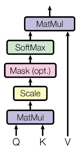
To compute this weighted sum, we first compute the attention matrix \(QK^T\). This matrix is of shape \((N, N)\). This is the source of the \(N^2\) complexity of transformers. The attention matrix contains scores for every combination of token query and key embeddings: \(q*k\), which is scaled by a factor \(\frac{1}{\sqrt{d_k}}\). This scaling is applied to normalize the gradients, such that the magnitude of the dot product isn’t dependent on the embedding dimension. This specific attention formulation is called scaled dot-product attention.

A softmax is applied to each row or column, creating a weight vector for each token. This is multiplied by the value matrix to generate a weighted sum for each token. Because all matrices are learned, each token can determine which tokens to attend to, which tokens should attend to it, and what information to broadcast. This function is highly flexible. A token could even learn to nullify its own information and instead read from other tokens.

Self-attention is like a fully connected neural network layer in that information from all tokens can propagate to other tokens. However, self-attention has the benefit of supporting variable length input.

Cross-Attention

Self-attention is a mechanism where queries, keys, and values all derive from the same set of input embeddings. In contrast, cross-attention operates on two distinct sets of embeddings, which can have different lengths. The queries come from one set, while the keys and values come from another.

In cross-attention, the attention matrix \(QK^T\) is of shape \((N_Q, N_K)\) . \(N_Q\) is the sequence length of the queries, and \(N_K\) is the sequence length of keys. The softmax is taken on the rows, so each query token has a probability distribution with respect to keys.

Cross-attention is particularly relevant for machine translation. In this context, the keys and values come from the source language text, while the queries come from the target language. As the model generates the translation, it attends to the set of tokens from the source language, allowing it to draw information from the original text throughout the translation process.

Masked Self-Attention

The transformer decoder uses causal masking. The decoder is trained to predict the next token. This task becomes trivial if the next token and all future tokens are visible, as in full self-attention. Causal masking constrains the attention operation to only look at tokens to the left, making the decoder auto-regressive (meaning each output depends only on previous outputs). This one-way flow of information is essential for generating sequences one token at a time.

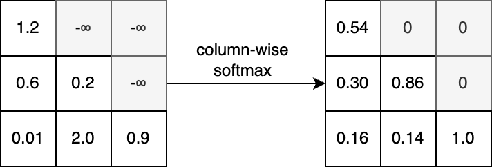
Masking is applied on the \(QK^T\) matrix. Masked indices are set to \(-\infty\), this causes the softmax function to assign zero weight to these tokens. In many implementations of attention, the mask can be customized by passing in a Boolean matrix.

Multi-Head Attention

Multi-head attention (MHA) is a way to increase the expressivity of the attention operator. It is essentially running multiple attention operations in parallel and concatenating the output. This improves expressivity because each head is free to attend to different tokens.

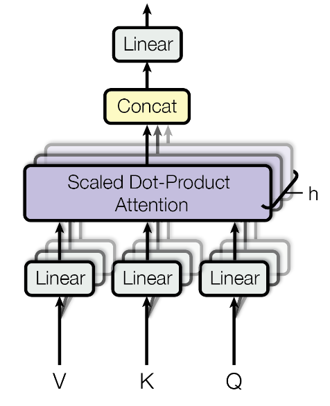
Multi-head attention has two scaling parameters. Feature dimension for each head \(d_v\), and number of heads \(h\).

Each head projects the input embeddings into queries, keys, and values of size \(d_v\). This means that the weight matrices \(W^Q\) , \(W^K\), and \(W^V\) are of size \((d_{model}, d_v)\). Attention is applied to the set of queries, keys, and values independently. This results in \(h\) sets of output embeddings of size \(d_v\). The output embeddings of each head are concatenated resulting in embeddings of size \(d_v*h\). The output needs to be the same dimension as the input, so there is linear projection back to size \(d_{model}\).

Typically the embedding dimension to each head is \(d_v = d_{model}/h\). In this case, the concatenated output is the same dimension as the input token embeddings. However, it is possible to set \(d_v\) to be higher or lower.

The output projection, which is a linear layer \(W^O\), learns to combine the outputs of the different heads. The output size of this layer is the same as the input token embedding size. This layer allows the model to give different importance to different attention heads. When \(d_v\) is set to \(d_{model}/h\), this projection is not required for dimensionality matching. However, it is beneficial in that the information from different heads can be mixed before the residual connection.

Multi-head attention (MHA) effectively divides the softmax operation into separate parts. Each head has a fixed amount of attention weight to distribute among different value functions. This multi-headed approach allows for more complex token interactions. One of the advantages of the attention mechanism is its interpretability. For each head, it’s possible to examine which tokens are attending to which other tokens, providing insight into the model’s internal workings.

Normalization

In transformer architectures, layer normalization is typically used. Unlike batch normalization, the values are independent of other items in the batch. This is because batch-wide statistics aren’t used. Layer Normalization was introduced just a year prior to transformers.

For each set \(x\) in the batch, the mean \(\mu(x)\) and variance \(\sigma(x)^2\) of the embedding values (across all ⁍ values of each embedding) are calculated. These values are used to normalize each embedding value:

\[\mathrm{LN}(x) = \frac{x-\mu(x)}{\sqrt{\sigma(x)^2+\epsilon}} *\gamma +\beta\]

\(\gamma\) and \(\beta\) are learned scalar parameters. \(\epsilon\) is a small constant used for numerical stability.

Layer norm is effective for multiple reasons. Since batch statistics aren’t used, it makes data parallelism more efficient. This is because the batch statistics do not have to be communicated between GPUs. LayerNorm is also not affected by the size of the batch, which means different batch sizes can be used at different times.

In Attention Is All You Need, the layer normalization occurs after each attention and feed-forward layer (Post-LN architecture). However, it is now more popular to put the layer normalization before these layers (Pre-LN architecture). This paper from 2020 shows that the Pre-LN architecture generally performs better. This is the only fundamental change to the original transformer architecture.

Feed-Forward

After each attention layer, a small feed forward neural network processes each token embedding. This is a position-wise operation. In the original paper, this is a two layer network with a ReLU activation after the first layer. The first layer outputs a dimension \(d_{ff}=2048\). The second layer projects these embeddings back to the original token embedding dimension \(d_{model}=512\). The first layer is set to the 4x the size of the token embedding. This multiplier is arbitrary but is considered to be an effective value given the efficiency tradeoff.

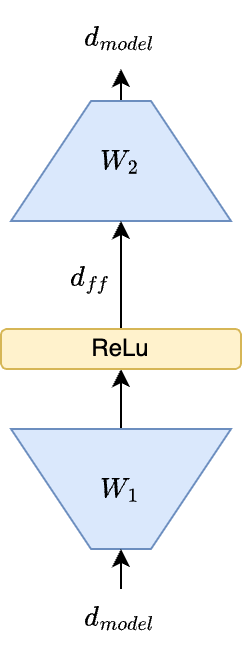
The attention layer has \(4*d_{model}*d_{model}\) parameters (accounting for query, key, value, and output projection matrices), which is \(1.0*10^6\) for the default embedding size. The feed forward layer has \(d_{model}*d_{ff} + d_{ff}*d_{model}\) which is over \(2.1*10^6\) parameters with the default configuration. When \(d_{ff} = 4*d_{model}\), this is equivalent to \(8*d_{model}*d_{model}\). The feed forward layer has roughly twice the number of parameters.

The attention layer computation scales quadratically with input length (default value is \(n=1024\)). The computational complexity of the feed forward layers is \(n*d_{model}*d_{ff}\). For attention, it is \(n^2d_{model}+d_{model}*d_{model}\). A recent trend is increasing the sequence length \(n\), which causes the attention layer to further dominate the computational cost. Due to the complexity of the attention operation and the different ways to implement it on hardware, we will skip calculating numerical values of the computation.

The feed forward layers contain the bulk of the transformer’s parameters, while the attention layers have the bulk of the computation. Attention is meant to learn the relationships between tokens, while the feed forward layers are meant to learn the individual token representations themselves. The attention operation is computationally intense in modeling the relationships between tokens, but it does not process individual token embeddings as much. The feed forward layers complement attention by enabling complex transformations of these embeddings.

This paper by Geva et al. argues that the feed forward layers act as key value memories. The high parameter counts of these layers enable the model to store rich information about the data they are trained on. Models like GPT-4 may not have their impressive world knowledge without the storage capacity of the feed forward layer. The transformer is a powerful architecture due to its balance of computational complexity and high parameterization.

Blocks

Now that we have covered each component, we can describe the transformer blocks. There are three main types of transformer blocks: encoder, decoder with cross-attention, and decoder without cross-attention. These blocks can be repeated any number of times.

Encoder Block

The encoder block maps a set of embeddings to another set of embeddings. It uses full self-attention, so each token can attend to all other tokens.

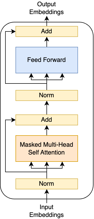
Decoder Block

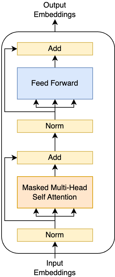
The decoder block takes in a set of input embeddings but also attends to a set of embeddings from the encoder. The first attention layer processes input embeddings with causal attention. The second attention layer is cross-attention, where the keys and values come from the encoder output. This kind of block is only used in encoder-decoder architectures since it relies on the encoder output embeddings.

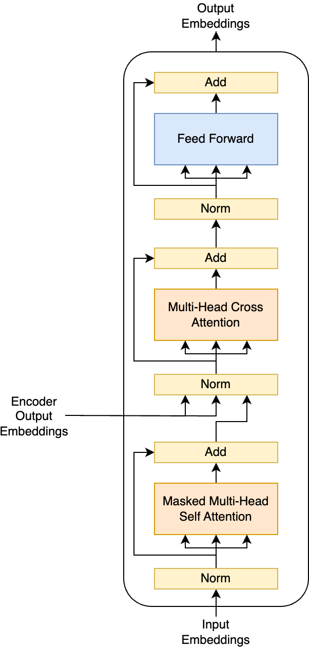
The cross-attention block is omitted in decoder-only transformers. This is because there are no encoder tokens to attend to. This block is identical to the encoder block, but the attention is masked.

Encoder-Only, Decoder-Only, and Encoder-Decoder Architectures

The original transformer paper introduced an encoder-decoder architecture. Since then, encoder-only and decoder-only architectures have gained significant popularity for various use cases. You can even have “encoder-heavy” or “decoder-heavy” architectures where one part of the transformer has more layers than the other. Let’s explore the different types of transformer models and their applications.

Encoder-Decoder

The encoder-decoder architecture can be viewed as two interconnected transformers. An encoder, which is a stack of encoder blocks, maps a sequence of input embeddings to output embeddings. A stack of decoder blocks with cross-attention then processes these embeddings. The decoder blocks read the final output embeddings from the encoder in the cross-attention layer.

The encoder and decoder can process different types of data. For instance, in speech recognition, the encoder might encode audio while the decoder translates it into text.

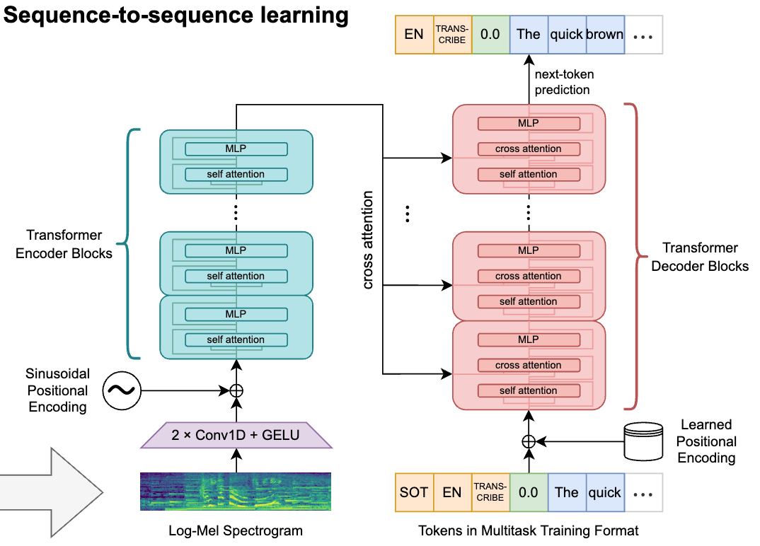
This architecture employs cross-attention, whereas encoder-only and decoder-only architectures rely solely on self-attention.

Encoder-Only

Encoder-only transformers, popularized by BERT, perform a one-to-one mapping of input embeddings to output embeddings. They can’t perform sequence-to-sequence modeling unless the input and output sequences have identical lengths.

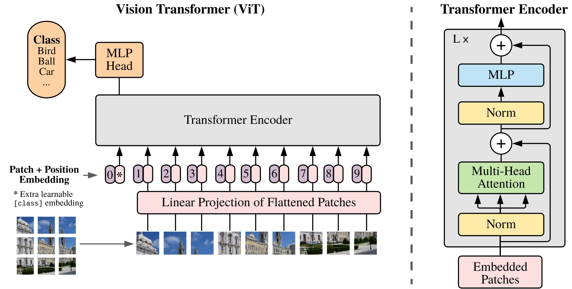
These models excel at scalar prediction tasks, such as classification or regression, where the output is a single value rather than a set or sequence. Text sentiment analysis and ImageNet classification are prime examples of their application.

Encoder-only models are useful in tasks reducible to token classification. For instance, BERT’s evaluation on the Stanford Question Answering Dataset (SQuAD) doesn’t generate text answers but identifies the relevant span in the input text. The task becomes classifying which tokens mark the start and end of the answer span. Similarly, Vision Transformer (ViT), another encoder-only architecture, is trained for ImageNet classification.

Decoder-Only

Decoder-only transformers have become the go-to architecture for Large Language Models (LLMs), popularized by OpenAI’s GPT models.

A decoder-only model can tackle any task an encoder-decoder can handle. Instead of processing source data through a separate encoder, all data flows through the decoder. The decoder omits the cross-attention layer since there’s no encoder to attend to. Its architecture mirrors that of the encoder-only transformer, with the key difference being causal attention.

The encoder-decoder architecture can be viewed as a constrained version of the decoder-only architecture. The separate encoding of source data in encoder-decoder models represents a form of inductive bias that decoder-only architectures generalize away from.

Encoder-decoder models require paired source and target text sequences for training, which can limit their flexibility. In contrast, decoder-only models can process a single input sequence, making them more versatile and adaptable to various tasks.

Decoder-only architectures have surpassed encoder-decoder models in popularity due to their simplicity and versatility. However, encoder-decoder models still offer unique advantages, such as the ability to train on encoder-specific objectives or fine-tune the encoder for downstream tasks.

Output Processing

The architecture of the output processing is simple. There is a final linear layer that maps embeddings of \(d_{model}\) to the size of the prediction. The output of the linear layer and how it is applied depends on the task the model is trained on.

Transformer models can be trained with different objectives and losses based on the use case and architecture type. We will discuss different types of objectives and how they are used for training. We will also explain how inference works under these objectives.

Next Token Prediction

Encoder-Decoder and Decoder-only transformers are primarily trained on next token prediction. This task involves predicting the subsequent word in a sequence based on the preceding words. The output layer is applied to each embedding, with the output size matching the input vocabulary size. A softmax function then creates a probability distribution over the token vocabulary, from which the next token is sampled.

During training, the decoder learns to predict the next word given the context. Causal masking ensures that for each token, the model can’t see the next or subsequent tokens in the sequence.

For each token, the ground truth preceding tokens are used as context. This is known as teacher forcing, as the generated tokens aren’t used as context. However, at inference time, autoregressive decoding is used instead. We start with a context—a set of input tokens. For chatbots, this might be the user’s input; for translation, the source text. The model predicts the next token, which is then added to the context, and another token is sampled. This process iterates until a special token is produced or a predetermined limit is reached.

At each step, the model outputs a probability distribution for the next token. This allows for sampling random sequences with a tunable temperature parameter, a common input for LLM APIs. Other decoding methods, such as beam search, can also be employed.

Next token prediction training is highly parallelizable. A single forward pass generates predictions and losses for each token in the input. However, inference is an iterative process requiring a forward pass for each generated token.

Masked Language Modeling

Masked Language Modeling (MLM) is a training objective introduced by BERT. This method trains encoder-only transformers. MLM training follows these steps:

1. Randomly select 15% of the input tokens for potential masking.
2. Of these selected tokens:
   • • 80% are replaced with a special [MASK] token
   • • 10% are replaced with a random token
   • • 10% are left unchanged
3. Apply the linear output layer to all masked predictions. Use cross-entropy loss to predict the correct token, regardless of how it was masked.

The intuition behind this technique differs fundamentally from next token prediction in that it’s bidirectional. As it’s an encoder-only architecture with full self-attention, tokens to the left and right are used to predict the masked tokens accurately.

MLM is a pretraining method that doesn’t yield directly interpretable output. The model can be used for embedding representations, where the output embedding is aggregated and used in another application. The model can also be fine-tuned on a scalar prediction task.

Scalar Predictions

Encoder-only transformers support a wide variety of losses in addition to MLM. While MLM is a per-token objective where outputs are generated from multiple tokens, many objectives require using an output linear layer on a singular embedding to get a single output.

There are multiple ways to achieve this:

• • Special output token
  • BERT and ViT add a token to the input. The output embedding from this input is used for predictions.
• • Output pooling
  • Alternatively, you can take the average of all the embeddings and apply the output layer on this pooled embedding.
• • Attentive probing
  • Attention can process the output. A learnable query vector attends to all token embeddings, producing a weighted sum that is then used for the output layer. This is essentially a cross-attention with a fixed number of query embeddings.

Once you have a singular output embedding, it can be processed by the output linear layer, and then any loss function relevant to the objective.

Conclusion

This blog post covered the basic components of early transformers. In part 2, we will cover more recent innovations that further optimize these models and enable new capabilities.