While the core transformer architecture introduced in “Attention is All You Need” remains effective and widely used today, numerous architectural improvements have emerged since its inception. Unlike the dramatic evolution seen in Convolutional Neural Networks (CNNs) from AlexNet onwards, transformer modifications tend to be more incremental and optional - the original architecture still serves as a strong baseline. This speaks to the elegant design choices made by the original authors, while leaving room for ongoing optimizations in efficiency, context length, and multimodal capabilities.

This post will focus on changes to the Transformer architecture that have been popular in the last couple of years (as of 2024). Time will tell which of these will be relevant in the future. For a deep dive on the original transformer architecture from Attention is All You Need (2017), see part 1 of this blog post. ML researchers and engineers use a lot of jargon when discussing transformers. This blog post seeks to elucidate it.

The original transformer architecture is very powerful and can handle a very wide range of applications. However, there are some limitations that more recent research has sought to address:

Long context
- Transformers are limited by their \(N^2\) computational complexity. This limits the sequence length a transformer can process, especially under resource and latency constraints.
Multimodality
- While transformers were originally developed for language processing, which remains their primary application, they have since expanded to handle nearly all data modalities and power large multimodal models.
Efficiency
- Scaling is attributed to the recent successes of LLMs. To enable this scaling, the model architecture needs to be designed efficiently.
- There have also been some research into more efficient computation. The same operations can be rewritten to run faster on hardware.

This blog post will cover the modifications to the architecture that are popular in the ML community and are applied in cutting edge industry applications such as LLMs (GPT, Claude, Gemini). This will give the prerequisite knowledge to understand these SOTA models. Many of these optimizations are only popularly used in LLMs. I find that transformers in other modalities, such as vision transformers, tend to stick to more vanilla architectures and training procedures.

While these architectural improvements are significant, they aren’t the main driver of AI’s remarkable progress in recent years. The real paradigm shift has come from post-training techniques. Specifically, fine-tuning and instruction tuning methods have enabled us to leverage language models more effectively for a variety of use cases. I initially planned to cover these techniques here, but as this post grew longer, I realized they deserve a part 3 to do them justice. For now, we’ll focus purely on the architectural changes to the model itself.

Many of the topics covered in this blog are large and active areas of research. These may warrant their own blog posts to give the research justice. However, in this post, we will take a myopic view and not cover this breadth of research. This will allow us to focus on more aspects of modern transformer applications and how they relate to each other.

To understand the current state of the art, we will look at technical reports for foundational LLMs: GPT, Gemini, LLaMA, Claude. We will also look at recent papers in other modalities to see how the transformer is adapted or evolved for these use cases. However, we find that there are generally fewer architectural changes in other domains.

Unfortunately many of the most used transformer models are opaque in that the public has access to very limited details of their architecture. Even open source models usually only make the inference code open, while keeping the training code closed. However, the following models can still help us understand the current state of the art:

Open Source LLMs
- LLaMA (2023): LLaMA, LLaMA 2, LLaMA 3
- Gemma (2024): Gemma, Gemma 2
- Mistral (2023): Mistral 7B, Mixtral of Experts
- Qwen (2023): Qwen
- Phi (2024): Phi-3, Phi-4
- DeepSeek
- OLMo (2024): OLMo, OLMo 2
  - Open training code!
Text encoder LLMs
- ModernBERT (2024)
Open Source Vision Language Models
- PaliGemma (2023)
- DeepSeek-VL2 (2024)
Computer Vision Models
- ViT-22B (2023)
Many more!

Through looking at these technical reports, you find that they share many of the same architectural improvements. This blog seeks to explain these improvements. I believe it is likely that the closed source transformers (GPT 3+, Gemini, Claude) aren’t that different.

Normalization

In part 1, we covered Pre-LayerNorm. We also see in architectures such as GPT that layer norm is added before and after the feed-forward and attention layers. This change was introduced in GPT-2. Generally, adding more normalization is inexpensive and has little downside, but can significantly improve and speed up training.

There are also new types of normalization being used. RMSNorm is currently a popular variant, used in LLaMA.

To refresh, layer normalization is defined as follows:

\[\mathrm{LN}(x) = \frac{x-\mu(x)}{\sqrt{\sigma(x)^2+\epsilon}} *\gamma +\beta\]

RMSNorm is defined as:

\[\mathrm{RMSNorm(x)} = \frac{x}{\mathrm{RMS}(x)} \gamma, \quad \text{where} \quad \mathrm{RMS}(x) = \sqrt{\frac{1}{N} \sum_{i=1}^N x_i^2+\epsilon}\]

The notation we use for RMSNorm is changed to be more aligned to the LayerNorm notation. \(x\) and \(\gamma\) are both vectors, and the division by \(\mathrm{RMS}(x)\) is broadcasted to each element of \(x\). \(\gamma\) is a vector or learned scaling parameters for each value of \(x\). It is written as \(g\) in the RMSNorm paper.

The difference is that RMSNorm rescales the features, while LayerNorm rescales and recenters the features. RMSNorm is designed to be shift invariant and not depend on the mean or recenter the values in any way. The mean subtraction is dropped from the numerator. \(\beta\) is also dropped to avoid a learned recentering. In LN, variance \(\sigma(x)^2\) depends on the mean (\(\frac{\sum_{i=1}^{N}(x_i - \mu)^2}{N}\)). RMS is used in place of variance to be completely independent of the mean. RMSNorm is completely shift invariant.

RMSNorm is more efficient than LayerNorm. The memory usage is halved because there is only one learned parameter \(\gamma\), since \(\beta\) is dropped. There is also less computation since there is no mean subtraction. These small efficiency gains become significant when applied to transformers with hundreds of billions of parameters. Another possible advantage is that it also constrains the model less, while still keeping the advantages of normalization.

Activation Functions

The original transformer used ReLU activation functions, which appear only between the two layers of the feed-forward block. Since then, two other activation functions have gained popularity: GeLU and SwiGLU.

Research into activation functions remains largely empirical, with limited theoretical understanding of why certain functions outperform others. The research community has spent years optimizing every component of the transformer architecture, including the ReLU activation function. These functions should be considered for any new transformer application, but one should only expect a modest improvement in performance. Nevertheless, their mathematical formulations are quite interesting and worth understanding.

“We offer no explanation as to why these architectures seem to work; we attribute their success, as all else, to divine benevolence.” - Noam Shazeer in “GLU Variants Improve Transformer”

Gaussian Error Linear Units (GELUs)

GeLU is formally defined as follows:

\[\mathrm{GeLU}(x)=xP(X \leq x)=x\Phi(x)\]

\(\Phi(x)\) or \(P(X \leq x)\) is the standard Gaussian cumulative distribution function (CDF). It is the probability of values less than \(x\) occurring in a standard normal distribution: \(\Phi(x)=P(X \leq x); X\sim\mathcal{N}(0,1)\). GeLU multiples the input by this probability.

The CDF is defined as follows:

\[Φ(x) = (1/2) * [1 + \mathrm{erf}(x / √2)]\]

The error function is defined as:

\[\text{erf}(x) = \frac{2}{\sqrt{\pi}} \int_{0}^{x} e^{-t^2} dt\]

The integral in \(\mathrm{erf}\) needs to be approximated for practical use. There are two ways to approximate GeLU:

\[\mathrm{GeLU}(x)\approx0.5x(1 + \tanh[\sqrt{2/π}(x + 0.044715x^3)])\] \[\mathrm{GeLU(x)} \approx x\sigma(1.702x)\]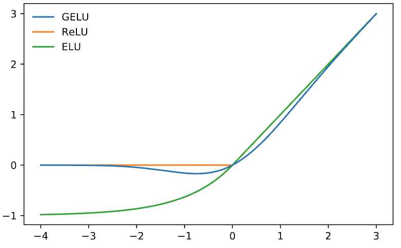

GeLU can be interpreted as a smooth version of ReLU with the added property of non-zero gradients for negative inputs.

The GPT-2 code uses the longer and more exact approximation. The shorter approximation is much more computationally efficient. Nowadays, this is more popular because the difference in model performance is negligible.

GeLU is used in BERT and GPT models. It is also popular for vision transformers such as ViT-22B.

SwiGLU

SwiGLU builds on the Swish activation function. This is also referred to as SiLU (Sigmoid Linear Unit) in the GeLU paper.

\[\mathrm{Swish}(x) = x\sigma(x) = \frac{x}{1+e^{-x}}\]

SwiGLU is a gated linear unit (GLU) version of this. GLUs were introduced in 2016. GLUs modify the feed-forward network by introducing a gating mechanism that controls information flow, allowing the network to selectively emphasize or suppress different parts of the input. This works by adding another linear transformation of the input \(Vx\) that acts as the gating function. The gating function performs element-wise multiplication with the output of the first feedforward layer and activation function. SwiGLU is a GLU that uses Swish as the activation function.

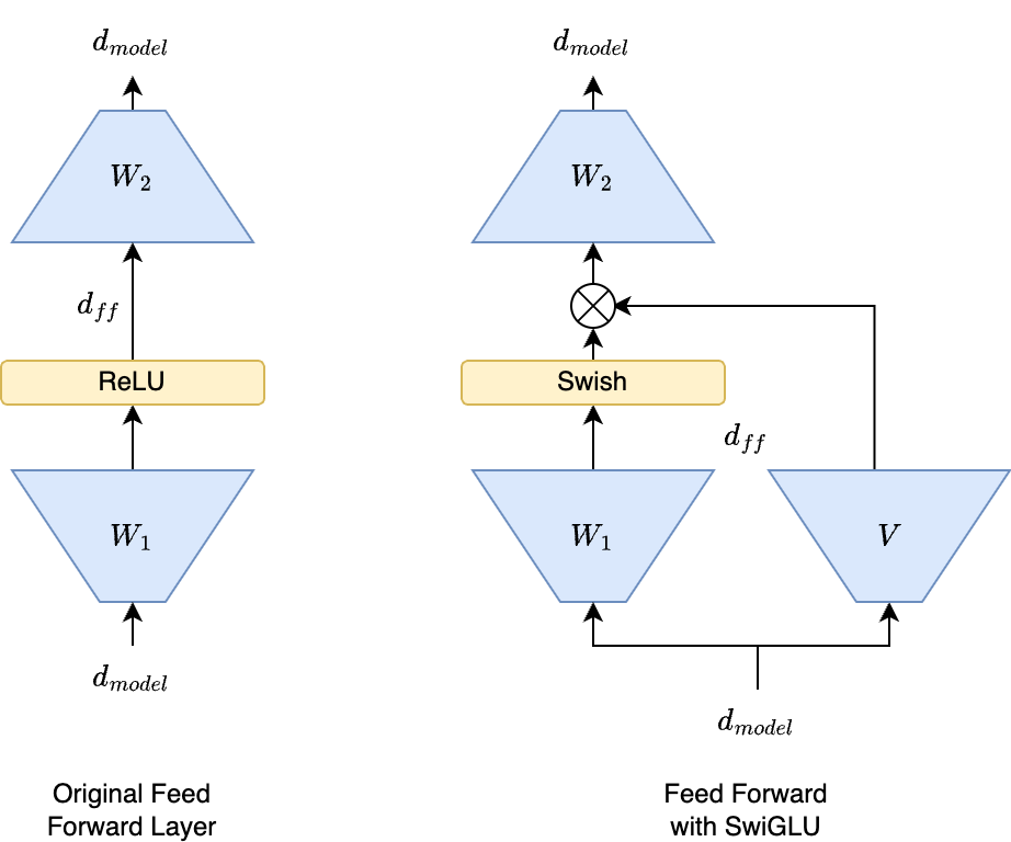
\[\mathrm{SwiGLU}(x) = \mathrm{Swish}(xW_1+b)⊗(Vx+c)\]

GLUs are more expensive since \(V\) is essentially a third linear layer in the feed-forward block, the same size as \(W_1\). To ameliorate this cost, the SwiGLU paper sets \(d_{ff}\) to \(\frac{2}{3}4d_{model}\), instead of \(4d_{model}\). \(\frac{2}{3}\)is chosen to keep the total number of parameters in the feed-forward block constant, since we have three weight matrices of the same parameter count instead of one. LLaMA also uses this ratio. However, this additional matrix multiplication is in parallel to the first linear layer. Depending on the hardware, it may have negligible training speed implications. The gating mechanism improves the performance of the model enough to warrant a reduction in the width of the feed-forward block.

GLU also increases the expressivity of the linear layer. The first linear layer is able to represent second order polynomials like \(x^2\), due to the element-wise multiplication. This may compensate for reduced width.

SwiGLU is used by many recent LLMs such as Mixtral/Mistral, LLaMA, and Qwen. Gemma uses GeGLU, which was introduced in the same paper as SwiGLU (GLU Variants Improve Transformer). GeGLU is a gated linear unit (GLU) variant of GeLU (GELU in place of Swish).

Position Embedding

In part 1, we covered two basic implementations of position embeddings tested in the “Attention Is All You Need” paper: learned position embeddings and sinusoidal position embeddings. These absolute position embeddings are functions of each token’s position in the sequence. While these methods are straightforward, they have notable limitations.

One key challenge is generalizing position embeddings to longer context lengths than those used in training. LLMs are typically pretrained with a fixed context length (e.g., 4096), but we often want to use them with longer sequences during inference. Learned position embeddings can’t generalize beyond their training sequence lengths since they lack embeddings for later positions. This is why sinusoidal position embeddings, which can naturally extend to any length, have become more popular.

Another limitation is that absolute position embeddings are permutation invariant, which isn’t ideal for many applications. This has led to research into relative position embeddings, which encode the positional relationship between pairs of tokens rather than their absolute positions in the sequence.

Relative Position Encoding

Relative position encoding (RPE) uses the distance between tokens to define an embedding. Absolute position embeddings are simple in that they only require adding an embedding to the input token embeddings of the model. Each token maps to one embedding. With relative position embeddings, there is an embedding for different pairs of tokens. This requires computing the embeddings in the attention operation.

For a sequence of length n, there are \(2n-1\) different pairwise distances ranging from \(-n/2\) to \(n/2\), including 0. The distance can also be clamped by a max distance to reduce the number of parameters. These distances are mapped to learned embeddings.

RPE was introduced by Shaw et al. 2018. This particular implementation can be referred to as the Shaw relative position embedding. Rather than using matrices, the paper describes how individual attention scores, for query token \(i\) and key token \(j\).

The following equation describes how relative position is encoded into attention:

\[\begin{equation}e_{ij} = \frac{(x_i W^Q)(x_j W^K+a_{ij}^K)^T}{\sqrt{d_z}}\end{equation}\] \[\begin{equation}z_i = \sum_{j=1}^{n} \alpha_{ij}(x_jW^V + a_{ij}^V)\end{equation}\]

Equation (1) describes how the attention scores are calculated. Equation (2) shows how relative position is encoded into the values. It essentially reweighs the values based on relative positions. \(\alpha\) is just \(e\) after softmax along the key dimension. The change from standard attention is the addition of \(a_{ij}^K\) and \(a_{ij}^V\). These are learned embeddings that bias the keys and values based on the relative position between \(i\) and \(j\). The bias on the key is different based on which query it will be in a dot product with. The embedding lookup is based on the difference between \(i\) and \(j\) and a max distance parameter \(k\). There are separate embedding tables for keys and values: \(w^K\), \(w^V\).

\[\begin{align*} a_{ij}^K &= w^K_{\text{clip}(j-i, k)} \\ a_{ij}^V &= w^V_{\text{clip}(j-i, k)} \\ \text{clip}(x, k) &= \max(-k, \min(k, x)) \end{align*}\]

Relative position is encoded in the keys so that the attention matrix can capture positional relationships between tokens. The position can also be encoded in the values, so that positional information can be encoded in the embedding themselves. This makes sense since the attention mechanism is an information bottleneck since the scores are scalars, whereas values are embeddings. However, the paper reports that they get the best results from only adding relative position the keys. Relative position on the values does not add any additional performance but comes with an efficiency cost. We see subsequent works drop this term and focus on incorporating relative position in the attention matrix.

Now that we have defined how we can incorporate relative position within the attention operation, we must understand how to efficiently implement this. The notation above doesn’t use matrix multiplies and we cannot naively iterate over \(i\) and \(j\) with for loops. To implement the Shaw relative position embedding, \(a^K\) and \(a^V\) are computed as two matrices of size \((N, N, h, d_k)\) and \((N, N, h, d_v)\), result in \(O(N^2hd)\) memory utilization. The memory usage is reduced to \(O(N^2d)\) by sharing these embeddings between each attention head (this is also in line with absolute position embedding). The notation above disregards the attention heads dimension for simplicity. We can formulate attention with relative position as follows:

\[\text{RelativeAttention} = \text{Softmax}\left(\frac{QK^T + S^{rel}}{\sqrt{d_k}}\right)V\]

\(S^{rel}\) represents the relative attention bias which is calculated by initializing a matrix of size \([N,N,h,d_k]\). This contains embeddings of size \(d_k\) from each pair of \(N\) positions. This matrix adds significant memory complexity and contains repeated embeddings.

Huang et al. 2018 introduce in their Music Transformer paper another optimization to RPE to bring the memory complexity down to \(O(Nd)\). The key intuition is that there are only \(2n-1\) or \(O(N)\) possible relative positions possible. The Shaw RPE matrices include many duplicate embeddings because the same pairwise distances repeat many times in the model. We can restructure the computation so that these repeated embeddings aren’t stored in memory at the same time. This implementation does not include relative position in the values.

Music Transformer optimizes this by multiplying each query directly with the relative position embedding matrix: \(QE^{r\top}\). This produces a matrix of size \([N,N]\), matching the expected size of the attention matrix bias. \(E^r\) represents the embedding table as a matrix storing representations for every relative position (pairwise position difference). The matrix is then transformed into the correct attention bias \(S^{rel}\) through a series of operations which they refer to as a skewing procedure. While these transformations are confusing, the key point is that we avoid creating any \(O(N^2d)\) matrices. Instead, \(E^r\) only requires \(O(Nd)\) additional space, with all other matrices matching the attention matrix size of \(O(N^2)\).

Mask the top left triangle, this will be shifted to result in a causal mask
Pad an empty “dummy” column on the left side
Reshape the matrix from \([L,L+1]\) to \([L+1,L]\)
1. Row-major ordering would cause this to result in the values to be shifted such that the relative positions are aligned to the diagonals.
Remove the empty first row through slicing

Since relative position is encoded into the attention layers, it possible to use it alongside absolute position embeddings. Relative position embeddings are only required to be used in the first attention layer, since the information can propagate to subsequent layers. However, it is more common to use relative position attention in all of the transformer blocks. This may ensure that the position information is not disregarded by the model. It is much less common to add absolute position embeddings in every block.

Relative position embeddings add an inductive bias of translation invariance to the models. Given the scale of the datasets modern transformers are trained on, it seems like this bias would limit the model’s ability to learn. However, as with many results in this post, relative position embedding has empirical advantages in language modeling.

Attention Biasing

Relative position embeddings initialize embeddings for each relative position. However this can be simplified by mapping each relative distance to a scalar bias to the attention scores.

ALiBi

Attention with Linear Biases (ALiBi) is another method of position embedding introduced by Press et al. 2021.

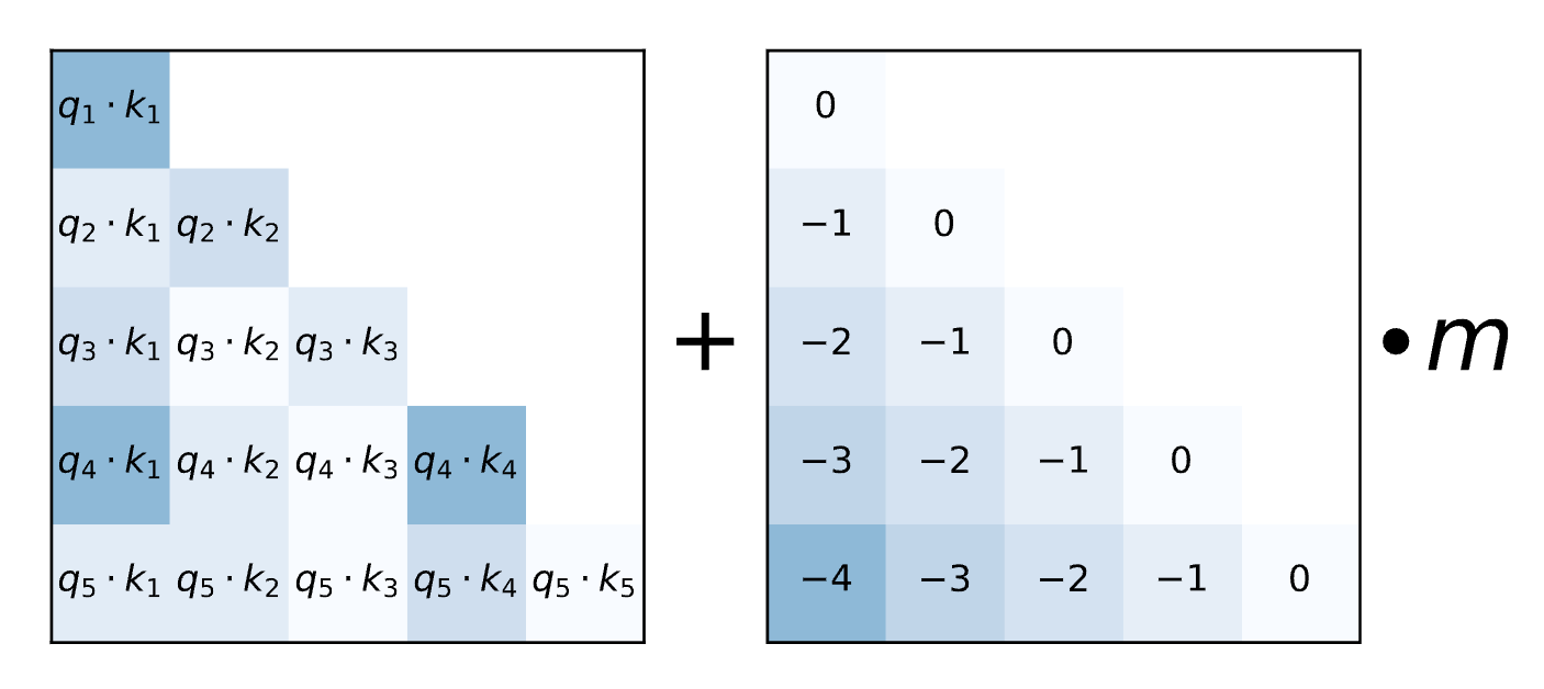
\(m\) is a hyperparameter that can be set per attention head. No absolute position embeddings are added. This method adds a strong inductive bias for locality. The attention scores decay with relative distance. Since there are no learned parameters for position this bias can generalize to longer sequence lengths during inference. The biases can be extended indefinitely.

T5

The T5 models introduced by Raffel et al. 2019, also utilize relative biases, but make these learned parameters that are shared among all the layers. Rather than setting a single hyperparameter \(m\), each relative distance maps to a learnable scalar bias value. This is more parameter efficient when compared to RoPE since the biases are shared across all layers, and they are scalars rather than embeddings.

RoPE

While relative position embeddings improve model performance, they require modifying the attention operation with position bias, adding computational complexity and memory overhead. Rotary Position Embedding (RoPE), introduced in the RoFormer paper by Su et al. 2021, offers an elegant solution by encoding relative position directly into the queries and keys. This approach keeps the attention operation unchanged by leveraging mathematical properties to achieve the same benefits more efficiently.

The attention matrix contains dot products between query and key embeddings: \(\langle q_m,k_n \rangle\) . The key property of relative position embeddings is that this dot product does not depend on the absolute positions \(m\) and \(n\), but rather the relative position \(m-n\). This is translation invariant, meaning that the output is the same if you shift \(m\) and \(n\) by any constant amount. RoPE exploits the fact that we do not care what information is in the queries and keys, we only care about the dot product.

\[\langle f_q(x_m,m), f_k(x_n,n) \rangle = g(x_n, x_n, m-n)\]

RoPE groups the embedding dimensions into groups of two adjacent indices. These two values can be considered to be defining a complex number. The first number represents the real part, and the second is the imaginary dimension.

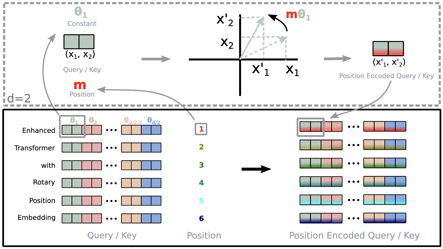
If the embeddings are of size \(d\), \(d/2\) of these size two blocks / complex numbers are present. The absolute position of the embedding in the input sequence is denoted \(m\).

Each of these groups representing a vector will be rotated. There is a different angle \(\theta\) of rotation for each position \(m\) from 0 to \(d/2\).

\[\Theta=\{\theta_i=10000^{-2(i-1)/d},i\in[1,2,...,d/2]\}\]

The value 10000 follows the sinusoidal position embedding in Attention Is All You Need and is equivalent to \(\theta_1\). Each group is rotated by the angle \(m\theta_i\). The rotation matrix is defined as:

\[\begin{bmatrix} \cos(m\theta_i) & -\sin(m\theta_i) \\ \sin(m\theta_i) & \cos(m\theta_i) \end{bmatrix}\]

Given that \(m\) is a variable index. The \(\theta\) values define frequencies. Each group’s vector is rotated at a different frequency. This helps the model learn short and long range relationships between tokens.

We want to multiply a vector containing \(d/2\) groups by different rotation matrices. To accomplish this, the different rotation matrices are placed on a diagonal. This matrix is sparse and the rotation can be efficiently computed.

\[R_{\Theta,m}^d = \begin{pmatrix}\cos m \theta_1 & -\sin m \theta_1 & 0 & 0 & \cdots & 0 & 0 \\\sin m \theta_1 & \cos m \theta_1 & 0 & 0 & \cdots & 0 & 0 \\0 & 0 & \cos m \theta_2 & -\sin m \theta_2 & \cdots & 0 & 0 \\0 & 0 & \sin m \theta_2 & \cos m \theta_2 & \cdots & 0 & 0 \\\vdots & \vdots & \vdots & \vdots & \ddots & \vdots & \vdots \\0 & 0 & 0 & 0 & \cdots & \cos m \theta_{d/2} & -\sin m \theta_{d/2} \\0 & 0 & 0 & 0 & \cdots & \sin m \theta_{d/2} & \cos m \theta_{d/2}\end{pmatrix}\]

We can multiply this matrix by the query \(Q\) and key \(K\) matrices to encode the positions. The standard attention formula can be applied to these rotated queries and keys. We have defined the rotation and the implementation of RoPE but now we’ll show how this actually encodes position.

Let’s take a arbitrary query embedding \(q_m\) and a key embedding \(k_m\). We can assume an embedding dimension of 2 so that the query and key map to only one complex number. The multiplication with the 2d rotation matrix is equivalent with multiplying with \(e^{im\theta}\) and \(e^{in\theta}\). Multiplying a complex number \(z = x + iy\) by \(e^{imθ}\) effectively rotates \(z\) counterclockwise by an angle \(m\theta\). \(x\) and \(y\) are the two components in the embedding group. Expanding the product:

\[\begin{aligned}e^{imθ} * z &= (\cos(mθ) + i*\sin(mθ))*(x + iy)\\ &=(x*\cos(mθ)-y*\sin(mθ)) + i*(x*\sin(mθ) + y*\cos(mθ))\end{aligned}\]

This is equivalent to multiplying with the 2d rotation matrix, assuming the first value \(x\) in the group represents the real component and \(y\) is the second and imaginary component.

\[\begin{aligned}R(θ) * [x, y] &= \begin{bmatrix} \cos(m\theta_i) & -\sin(m\theta_i) \\ \sin(m\theta_i) & \cos(m\theta_i) \end{bmatrix} * [x, y] \\ &= [x*cos(θ) - y*sin(θ), x*sin(θ) + y*cos(θ)]\end{aligned}\]

The query embedding is rotated by \(m\theta\) and the key is rotated by \(n\theta\).

\[q_m^r = q_m*e^{im\theta} \\ k_n^r = k_n*e^{in\theta}\]

In attention we are interested in the dot product of these rotated vectors. The dot product of the vectors is equivalent to the inner product of the complex numbers the 2d vector represents. The complex inner product is defined as \(Re[ab^*]\). We take the conjugate of the rotated key embedding:

\[k_n^{r*} = k_n^**e^{-in\theta}\]

We take the conjugate value of \(b\) and take the real part of the product. This can be applied to the query key product:

\[q_m^r*k_n^r = Re[q_m*e^{im\theta}*k_n^{r*}e^{-in\theta}] = Re[q_m^r*k_n^{r*}e^{i(m-n)\theta}]\]

This shows that we have reached our desired property that the dot product depends on the relative position \(m-n\), but not the absolute positions \(m\) and \(n\). This is also translation invariant in that you can shift \(m\) and \(n\) by a constant amount and not change this dot product.

Unlike RPE, RoPE doesn’t require modifying the attention operation. It just requires transforming the input query and key matrices. This makes RoPE easier to efficiently implement. RoPE also has no learned embeddings. Attention is All You Need shows that sinusoidal position embeddings, with no learned parameters, performs just as well as learned position embeddings. RoPE can be thought of as an extension of sinusoidal embeddings that prefers relative position information.

We’ll now revisit the \(\theta\) parameters to understand how they affect long context inference. \(10000\) can be considered the base frequency \(b\). This is an important hyperparameter that determines the lowest and highest frequency rotations. Given the embedding dimension \(d\), the lowest frequency rotation is \(\theta_{d/2} = b^{2/d-1}\). With the settings \(b=10000\) and \(d=768\), this corresponds to a wavelength of about 9763 tokens. This means for long context LLM inference (>32k tokens), this rotation would become periodic. ****This directly affects the sequence lengths that RoPE can handle effectively. If \(b\) is set too low, RoPE becomes periodic during longer context inference and performance suffers.

RoPE is still periodic like the sinusoidal absolute position embedding in the original transformer. However the difference is that it is periodic in the relative positions, not the absolute positions. The translation invariance significantly improves performance, but there is still room for improvement in the periodicity of the relative positions. Several approaches can be used to help RoPE perform better at long context inference.

Positional Interpolation

Tian et al. 2023 introduces a simple method to improve RoPE’s extrapolation capabilities. For models trained with context length \(L\) that need to handle longer contexts \(L'\) during inference, RoPE can be rescaled using:

\[\text{f}'(x,m)=\text{f}'(x,\frac{mL}{L'})\]

This rescaling reduces the rotation applied to each token embedding. Though this approach requires finetuning for the new context length, the authors show that just 200 finetuning steps yield strong results.

Another solution is to pretrain with scaled RoPE from the start. This approach was explored in Zhang et al. 2023 and implemented in Llama 3. By setting the base frequency \(b\) to 500,000, they achieved effective inference with context lengths of 32k. While this offers a simple solution, it may limit the model’s ability to learn proper processing of higher relative positions during training.

YaRN

Peng et al. 2023 improves on positional interpolation (PI) by scaling different RoPE frequencies differently. They hypothesize that PI hurts high frequency dimensions by changing the wavelengths by a significant portion. They adapt to this by scaling high frequencies less, and low frequencies more. As we previously discusses, the low frequency components are the most important to avoid periodicity.

This method in used in DeepSeek-V3 and Qwen2.

Additional Resources

Efficient Attention

The \(N^2\) complexity of self-attention has long been considered a major bottleneck. There has been a lot of research into sparse attention methods, such as BigBird and Sparse Transformers. While these methods enhance efficiency through sparse attention patterns, they come at the cost of model performance. Because of this, we don’t see these methods adopted in frontier LLMs.

Sliding Window Attention (SWA) is another sparse attention method introduced in Longformer. Instead of having a query token attend to all prior key tokens, it attends only to \(w\) (window length) prior tokens. This reduces attention complexity from \(N^2\) to \(Nw\). However, effective performance requires a substantial window length. For example, Mistral uses a window length of half the context length. This is implemented through an attention mask during training. During inference, the KV cache (explained later) size can be reduced from \(N\) to \(w\).

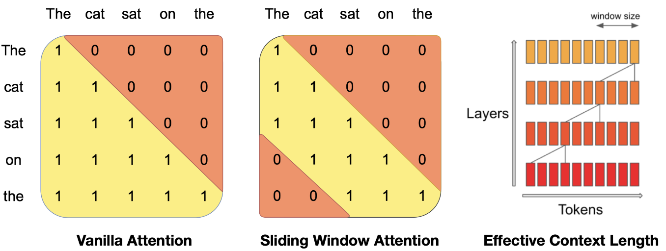
SWA resembles convolution in that tokens attend only to nearby tokens. Longformer employs smaller window sizes in earlier transformer blocks and larger ones in later blocks. This enables both local and global information flow, allowing learning at different scales—similar to CNN architecture.

A key limitation is that distant tokens cannot communicate directly. Information must flow through multiple transformer layers to connect distant tokens. To address this, models like Gemma 2 and ModernBERT alternate between SWA and global attention blocks. By maintaining global attention blocks throughout the network, distant token can still communicate quickly. We can adjust the number of SWA blocks and window size to manage this efficiency tradeoff.

SWA has emerged as a powerful and practical method for improving transformer efficiency. It has been gaining more traction in LLMs than other sparse attention approaches. SWA typically uses a large window size - usually half the global context length. This makes it more similar to global attention than sparse/local attention. However, it still offers substantial benefits. It halves both the KV cache size during inference. Additionally, it reduces the attention computation during both training and inference. SWA also avoids the issues of position embedding extrapolation by capping the maximum relative positions in the attention operation.

FlashAttention

FlashAttention (Dao et al. 2022) is an optimization to the computation of the attention operation. They are designed to be completely accurate in their results, but more efficiently run on GPUs. We will focus on FlashAttention-2, which has several significant improvements. FlashAttention-3 is another optimization, however, it is designed specifically for NVIDIA GPUs.

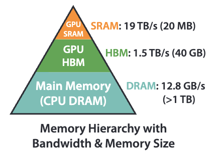
When designing algorithms like attention, we often only consider the number of floating point operations (FLOPs). However, we need to more carefully consider the hardware. Specifically, GPUs are very fast in computing highly parallelized floating point operations, but have slower memory access. We can speed up attention by reducing the amount of memory reads and writes, even if it comes at the cost of additional computation.

GPUs have two types of memory: slow but large HBM (high bandwidth memory) and small but fast SRAM (static random access memory). When working with large matrices, we load blocks (parts of the matrices) from HBM into SRAM. The computation takes place and then the output is written back to HBM.

We will review two prerequisite topics before covering FlashAttention.

Block Matrix Multiplication (BMM)

Block matrix multiplication enables matrix multiplications to be parallelized by splitting the inputs into blocks and concatenating output blocks. If we are trying to compute \(C=AB\), a certain output block requires a subset of rows from \(A\) and subset of columns from \(B\). We can just take the input blocks containing these rows and columns, rather than reading the entire matrix into memory.

\[A = \begin{bmatrix} A_{11} & A_{12} \\ A_{21} & A_{22} \end{bmatrix}, \quad B = \begin{bmatrix} B_{11} & B_{12} \\ B_{21} & B_{22} \end{bmatrix}\]

Each output block \(C_{ij}\) is computed using only the required blocks: \(C_{11} = A_{11}B_{11} + A_{12}B_{21}\). The shapes of these blocks need to be carefully defined to be compatible for the matrix multiplication, and be efficient on hardware. The number of rows in the blocks of \(A\) must match the columns of blocks of \(B\).

Computing an output block doesn’t require reading all the required input blocks at once. They can be read iteratively since it is a sum. When viewing matrix multiplication as dot products between rows and columns, the summation works by splitting these vectors into blocks, then summing the dot products of these blocks.

Parallel GPU cores can compute different output blocks while only reading the required input blocks. Attention is just two matrix multiplications \(S = QK^\top\) and \(O = P V\) and a softmax. FlashAttention takes advantage of the BMM algorithm to compute this more efficiently.

Online Softmax

With BMM, we can compute matrix multiplications block by block without needing any global information. However, there is a challenge in integrating softmax into this framework since it requires normalizations which need to be calculated globally from all blocks.

FlashAttention uses an online softmax to minimize the memory access. Recall the softmax operation:

\[\text{softmax}(x_i) = \frac{e^{x_i}}{\sum_{j=1}^n e^{x_j}}\]

The denominator \(l\) is the normalization factor. Also, softmax function is numerically unstable because exponents can reach extremely high values when \(x_i\) is a large positive number. To achieve numerical stability, we subtract the maximum value before computing the exponentials:

\[\text{softmax}(x_i) = \frac{e^{x_i - \max_j x_j}}{\sum_{j=1}^n e^{x_j - \max_j x_j}}\]

This subtraction keeps each exponent between 0 and 1, ensuring numerical stability. The result remains unchanged since this operation is equivalent to multiplying both numerator and denominator by the same constant. However, this maximum value is another global value.

A naive implementation would require 3 passes, one to find the max value, one to compute the numerator and accumulate the normalization factor, and one to apply the normalization factor. This requires a lot of memory access. However, we can optimize by fusing the first two steps into a single \(O(N)\) pass using this algorithm:

Assume the first element is the max \(m_j=s_{0j}\) and initialize an accumulator for the normalization constant as \(l_j := e^{s_{0j}-m_j}\)
Iterate through the rest of the list
1. If the value \(s_{ij}\) is less than or equal to the current max, add it to the accumulator: \(l_j := l_j+e^{s_{ij}-m_j}\).
2. If the value \(s_{ij}\) is greater than the current max, adjust the normalization factor (which was computed using the wrong max) by multiplying: \(l_j := l_j * e^{(s_{ij}-m_j)}\). This correction factor ensures \(s_{ij}-m_j\) is added to each incorrect exponent in the sum. Then update the max value: \(m_j:=s_{ij}\).
3. This entire update can be expressed without conditional logic: \(m_i := \max(m_{i-1}, s_{ij});\quad l_j := l_j * e^{(m_{i-1}-m_{i})} + e^{(s_{ij}-m_{i})}\)

Through this optimization, we’ve reduced the softmax computation from three linear passes to two. The correctness of this algorithm can be simply proved by induction. The method is defined as iterating over individual items in \(x\), however, it easily extends to iterating over blocks in \(x\). We compute the local softmax within the blocks and then accumulate a global normalization factor.

There are two main changes to attention implemented in FlashAttention: tiling and recomputation.

Tiling

We can reduce the number of memory reads and writes by fusing operations together. With two separate operations, the data will be read twice and written twice. If the operations can be fused together, there will be only one read and write. However, we have to consider that we are working with very large matrices and using highly parallelized computation. Block matrix multiplication along with online softmax enables us to compute attention in pass without writing the full matrix to memory.

With tiling, we restructure the attention operation to load data block by block from HBM to SRAM. The full attention matrix of size \((N,N)\) is never materialized at once or written to HBM. This is done by looping through the blocks multiple times to avoid the need to write to memory. This is increasing computation to reduce memory access.

With fused operations you are trading accessibility of the code for efficiency. Simple matrix operations for attention (like multiplications and softmax) are easy to understand and modify. However, when running attention at scale, implementing an optimized fused version makes practical sense. Currently, billions of dollars are being spent running attention. It is important that we make this operation as efficient as possible.

Recomputation

Typically, the attention matrix is stored in HBM during the forward pass for use in the backward pass. FlashAttention takes a different approach. It recomputes the attention matrix during the backward pass instead of storing it. While this requires computing the attention matrix twice, it eliminates the need to write the large matrix to memory.

The softmax normalization parameters from the forward pass are still stored, enabling the backward pass attention computation to be completed in a single pass.

logsumexp

For each example in the batch, we can save only one value for the softmax normalization instead of two. We need to save both the max value \(m_i\) and the normalization sum \(l_i\). We can store the logsumexp \(L_i = m_i+\log(l_i)\). We’ll show how we can compute a correct softmax with this.

\[\begin{aligned} \text{softmax}(x^{(j)}) &= \exp(x^{(j)}-L^{(j)}) \\ &=\exp(x^{(j)}-m^{(j)}-\log l^{(j)}) \\ &=\frac{\exp(x^{(j)}-m^{(j)})}{\exp(\log l^{(j)})} \\ &=\frac{\exp(x^{(j)}-m^{(j)})}{ l^{(j)}} \end{aligned}\]

This small trick reduces the memory writes from the forward pass by half.

Algorithm

Forward Pass

Iterate through query blocks to get \(\text{Q}_i\) (this step runs in parallel)
For each query block, iterate through key and value blocks to obtain \(\text{K}_j\) and \(\text{V}_j\)
1. Compute the attention block \(\text{S}_i^{(j)}=\text{Q}_i\text{K}_j^T\)
2. Update the maximum value \(m_i^{(j)} = \max(m_i^{j-1}, \text{rowmax}(\text{S}_i^{(j)}))\), where rowmax finds the maximum in the current block
3. Compute the unnormalized attention weights for the current block using the current maximum: \(\tilde{\text{P}}_i^{(j)}=\exp(\text{S}_i^{(j)}-m_i^{(j)})\)
4. Update the block output: \(\text{O}_i^{(j)} = \text{diag}(e^{m_i^{(j-1)}} - m_i^{(j)})^{-1} \text{O}_i^{(j-1)} + \tilde{\text{P}}_i^{(j)} \text{V}_j\)
  1. The first term adjusts the exponents from previous blocks
  2. This output remains unnormalized and contains only the softmax numerator
Normalize the output block and write to HBM: \(\text{O}_i=\text{diag}(l_i^{(T_c)})^{-1}\text{O}_i^{T_c}\)
1. \(T_c\) represents the final block index after completing the loop
Compute logexpsum and save to HBM for the backward pass: \(L_i = m_i^{(T_c)} + \log(l_i ^{(T_c)})\)

Backward Pass

Initialize gradient buffers in HBM for \(\text{dQ}\), \(\text{dK}\), \(\text{dV}\)
1. Initialize \(D=\text{rowsum}(\text{dO}\circ O)\) in HBM
Iterate through key and value blocks to obtain \(K_j\) and \(V_j\)
1. Initialize \(\text{dK}_j\) and \(\text{dV}_j\) in SRAM
2. Iterate through the output blocks and load \(\text{Q}_i\), \(\text{O}_i\), \(\text{dO}_i\), \(\text{dQ}_i\), \(L_i\), \(D_i\) to SRAM.
  1. Recompute the attention block \(\text{S}_i^{(j)}=\text{Q}_i\text{K}_j^T\)
  2. Normalize the attention using the saved logsumexp \(\text{P}_i^{(j)}=\exp(\text{S}_i^{(j)}-L_i)\)
  3. Calculate the following gradients
    1. \[\text{d}\text{V}_j \leftarrow \text{d}\text{V}_j + (\text{P}_i^{(j)})^\top \text{dO}_i\]
    2. \[\text{d}\text{P}_i^{(j)} = \text{dO}_i \text{V}_j^\top\]
    3. \[\text{d}\text{S}_i^{(j)} = \text{P}_i^{(j)} \circ (\text{d}\text{P}_i^{(j)} - D_i)\]
      1. This is derived from the Jacobian of the softmax
  4. Update \(\text{dQ}_i \leftarrow \text{dQ}_i + \text{dS}_i^{(j)}\text{K}_j\)
    1. This read from HBM and written back. This memory expensive step is necessary since we need to accumulate gradients for all query blocks before writing the final result
  5. Update in SRAM: \(\text{dK}_j \leftarrow \text{dK}_j + \text{dS}_i^{(j)T}\text{Q}_j\)
3. Write \(\text{dK}_j\) and \(\text{dV}_j\) to HBM

FlashAttention is a kernel fusion that torch.compile cannot find because it is a rewrite of the computation. NxN attention matrix is not materialized. This also allows larger values of N which is important for long context. It is now implemented in most deep learning frameworks.

FlashAttention achieves its performance improvements through careful memory management and tiling of the attention computation. Rather than computing the full attention matrix at once, it processes smaller blocks of queries and keys, reducing the peak memory usage. This optimization is particularly important for training and inference with long sequences, where the quadratic memory scaling of attention would otherwise be prohibitive.

Additional Resources

Mixture of Experts (MOE)

Mixture of Experts (MoE) is transformer architectural change applied to all of the feed-forward blocks. Rather than having one feed-forward module in each transformer block, there are multiple parallel feed-forward blocks. A gating network selects among these blocks. These blocks are considered experts that specialize in different things. Multiple blocks are selected and the output embeddings are added together, creating a mixture.

MoEs are considered to be sparse models. MoE models can have very high numbers of trainable parameters, but have only a fraction used for a given example during training and inference.

MoE is generally structured as follows:

Create \(n\) experts, which are separate versions of the feed-forward MLP block
A gating network / router processes the token embedding \(x\) and outputs a score for each embedding. This is a vector of size \(n\).
1. The gating network is typically implemented as a single learned MLP layer: \(W_gx\)
We select the top k experts and route the token embedding to these experts.
The output is a weighted sum between the outputs of the k selected experts
1. A softmax is used on the scores of the top k experts to normalize the weights

The number of selected experts \(k\) is chosen to be small (typically 2) to achieve this sparsity. With this approach and parameter setting, we achieve the goal of a sparse transformer architecture.

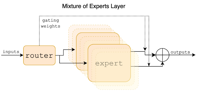
We want all \(n\) experts to be utilized with roughly equal frequency. In the worst case, the same \(k\) experts are selected for every input, and the remaining experts are just a waste of space. While each input should activate only a few experts, we want to ensure that all experts are activated with roughly equal frequency over the entire training set. We want to encourage diversity in expert selection. Different MoE implements achieve this differently.

Sparsely Gated MoE (2017)

Shazeer et al. 2017 introduces mixture of experts for language modeling, however, using LSTMs instead of transformers.

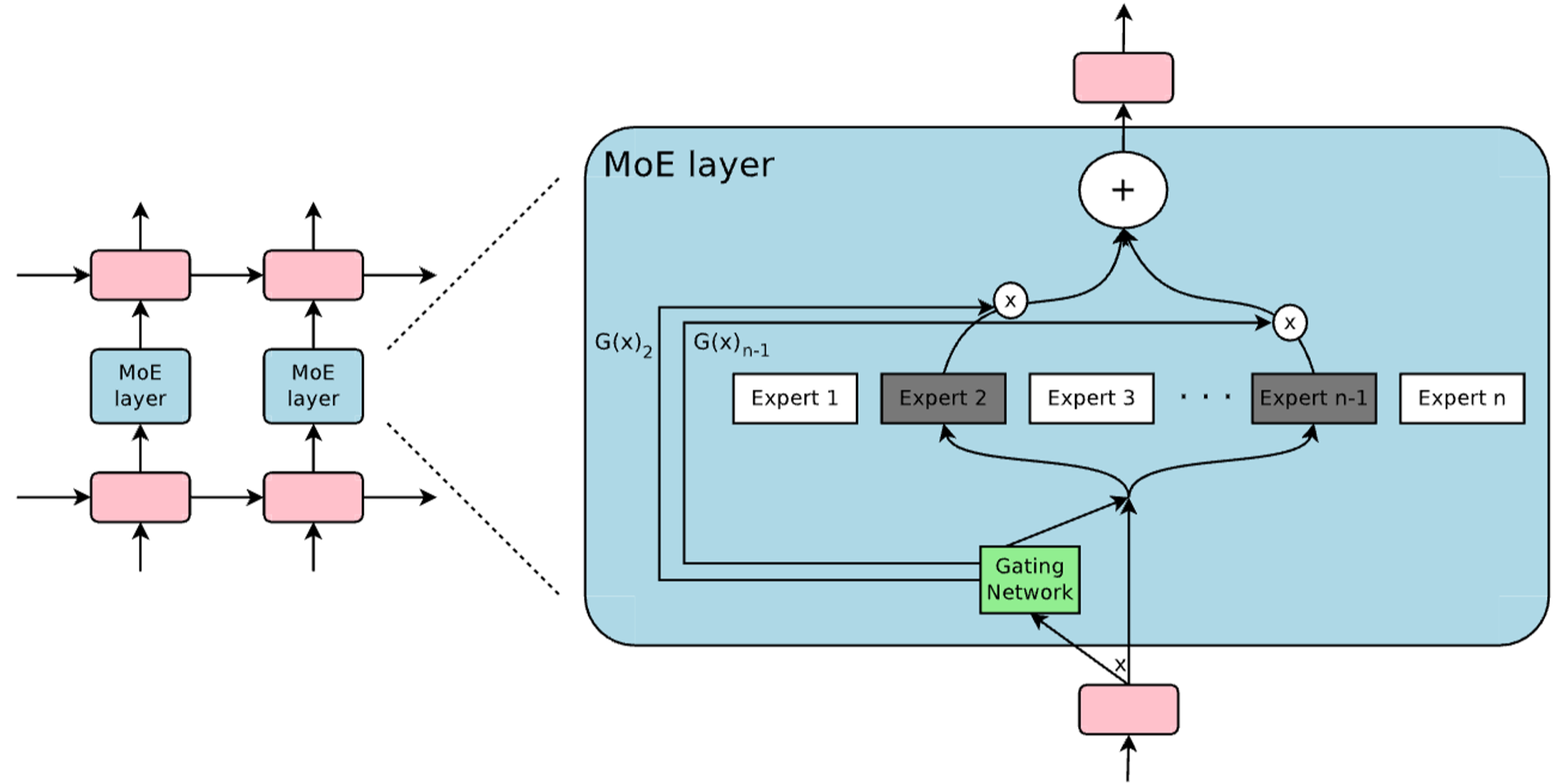
In order to enforce diversity, they add tunable Gaussian noise to the expert score \((xW_g)_i\) of each expert in the function \(H()\).

\[H(x)_i = (x \cdot W_g)_i + \text{StandardNormal()}\cdot \text{Softplus}((x \cdot W_{noise})_i)\]

The noise for each component is learned through \(W_{noise}\). A load balancing loss is optimizes the magnitude of the loss for different experts. Without a proper loss term, the noise would collapse to 0. This noise term is important for the load balancing loss.

Softplus is similar to ReLU but smooth and always non-negative: \(\text{Softplus}(x)=\log(1+e^x)\). This is just to make sure the noise added is non-negative.

After adding the noise, we apply the \(\text{KeepTopK}\) function. This sets the values to \(-\infty\) for experts outside of the top \(k\) to ignore them in the softmax. After the softmax, only two experts have weights, which add up to 1. The final weights on the experts is calculate as:

\[G(x) = Softmax(KeepTopK(H(x), k))\]

The softmax normalizes the weights of the two experts, which can be used to compute a weighted sum of the outputs of the selected experts.

For diversity, an additional importance loss term is used. Given an expert \(i\) and a training batch \(X\), we define importance as follows:

\[Importance(i,X)=\sum_{x\in X}G_i(x)\]

We then sum this across experts to define an auxiliary loss, which is minimized when all the experts are activated equally on the batch:

\[L_{importance,i}(X) = w_{importance} \cdot CV(Importance(i,X))^2\]

However, one shortcoming of the importance loss term is that it uses the weights. It is possible for an expert to have a high average weight, but never be selected in \(KeepTopK\). They define another loss \(L_{load}\) weighted by \(w_{load}\) to address this. We want a smooth estimation of the number of examples assigned to each expert. The definition of this is out of scope for this post, but it is designed to be smooth operation on a discrete operator.

A key challenge with MoE is that each expert only sees a fraction of the training batch, limiting its learning effectiveness. To address this, one solution is to use data parallelism with very large batch sizes.

MoE also requires careful handling in multi-device training setups. Through expert parallelism—a form of model parallelism—different devices manage different experts. After the gating function determines expert assignments, tokens are shuffled between GPUs in a ring pattern before returning to their original GPU. This allows us to use MoE to scale the number of parameters in a model, but there is an added communication cost with expert parallelism.

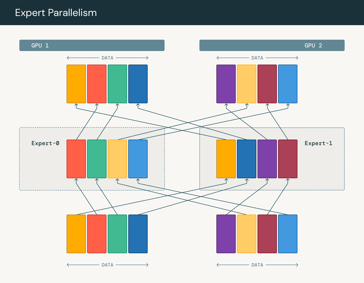
The auxiliary loss is calculated separately for each MoE layer in the transformer.

GShard

GShard (Lepikhin et al. 2020) applies MoE to transformer, also with k=2 experts. Each expert implements the same two-layer MLP architecture used in standard transformers. GShard uses a simpler auxiliary loss term to encourage expert diversity. It is simply \(\frac{c_e}{S}m_e\) where \(e\) is a particular expert. This loss is averaged across all experts. \(c_e/S\) is the fraction of the \(S\) tokens routed to expert \(e\). This is not differentiable because \(c_e\) is determined by the top k operator. This ratio acts as a weight on the mean weight of the expert \(m_e\) which is differentiable. The authors were able to train very large MoE transformer models while using this loss to balance tokens between experts.

The expert with the highest score is selected first. For the second expert, rather than choosing the next highest score, the system randomly samples from the remaining experts. This random selection promotes diversity, functioning similarly to the Gaussian noise term.

Switch Transformer

Fedus et al. 2022 applies MoE to transformers with some simplifications compared to the 2017 paper. They only use one expert by setting \(k\) to 1. Instead of having separate loading balancing and importance losses, they use one auxiliary loss term (same loss as GShard):

\[\mathcal{L}_{aux} = \alpha N \sum_{i=1}^{N} f_i P_i\]

\(f_i\) is the fraction of tokens routed to expert \(i\) and \(P_i\) is the fraction of router probability routed to expert \(i\). These are among all tokens in a batch. \(f_i\) is analogous to the load balancing loss and \(P_i\) is analogous to the importance loss. \(P\) is differentiable, while \(f_i\) is not. The loss works because \(f_i\) is treated as a weight on a differentiable loss. The multiplication with \(N\) ensures that the optimal loss is the same with different numbers of experts.

Frontier LLMs

Mixtral

MoEs gained significant popularity in LLMs with the Mixtral paper from Mistral AI. The model uses 8 experts but selects only 2 for each computation, with SwiGLU serving as the expert function. The MoE block operates as follows, where \(x\) represents input token embeddings and \(y\) represents output token embeddings:

\[y = \sum_{i=0}^{n-1} \text{Softmax}(\text{Top2}(x \cdot W_g))_i \cdot \text{SwiGLU}_i(x)\]

While the paper doesn’t detail the exact auxiliary loss, the Hugging Face implementation extends the Switch Transformer loss to work with any number of selected experts.

DeepSeek

DeepSeek shares more details in how they train their MoE models. They do not use an auxiliary loss. Instead, they add a bias term \(b_i\) to the scores of each expert. At the end of each training step, they update the biases by \(\gamma\), which they term as the bias update speed. If the expert is overloaded, the bias is subtracted. If it is underloaded, it is added. This is heuristic method that avoids the challenges of optimizing an auxiliary loss.

Although they don’t use an auxiliary loss for load balancing between experts, they do use one to encourage expert diversity within sequences. Their goal is for tokens within a single example to use different experts. This contrasts with other methods and challenges the intuition that experts should specialize in specific topics. They find empirically that this reduces expert specialization. They implement this similarly to the Switch Transformer loss but average the probabilities within a sequence. However, a recent paper by Wang et al. 2024 suggests this loss isn’t necessary for achieving expert diversity across sequences.

They also introduce the notion of shared experts. They have routed experts which are selected by a gating function. The shared experts are always used. These are meant to store more general knowledge, while the routed experts are more specialized. This requires having more experts activated if you want to have more than 1 routed expert. DeepSeek-V3 uses high numbers of experts (ex: 2 shared, 64 routed). To implement this efficiently, they implement each expert as a 2 layer MLP with a small hidden dimension.

MoE represents one of the most significant improvements to the transformer architecture. However, the research community has yet to converge on a standard implementation. Different papers approach expert diversity in varying ways. Understanding these documented methods provides a foundation for designing your own MoE model. The technique’s success has led to applications beyond language models into other domains, such as the Vision MoE (V-MoE) paper.

Additional Resources

Mixtral AI Talk
Mixture of Experts Explained - Hugging Face
Training MoEs at Scale with PyTorch
Why Llama 3 is not a MoE? - /r/LocalLLaMA
Bug from the Hugging Face Mixtral code explaining the auxiliary loss
Mixtral MoE inference code
DeepSeek-V3 MoE inference code

KV Cache

Modern transformer architectures have introduced several innovations to improve decoding efficiency, especially for handling long sequences and reducing memory usage during inference. These improvements are essential when deploying large language models in production environments with limited computational resources.

Decoding with an LLM involves two main steps:

Prefill: Processing the input prompt and prior context
Decoding: Generating new tokens

Efficiently Scaling Transformer Inference (Pope et al., 2022) explores how these decoding steps can be optimized. In language model decoding, both the context and previously generated tokens are needed to predict the next token. However, reprocessing these tokens from scratch would be inefficient. Instead, we can save the intermediate outputs of prior tokens to avoid recomputation.

Only the keys and values from the attention layers need to be preserved. Since transformer decoders use causal attention, new tokens don’t influence the embeddings of previous tokens. We can safely discard the query and output embeddings for prior tokens as they’re no longer needed for computation. The key and value embeddings are kept in the KV cache, allowing newly decoded tokens to attend to previous ones.

During the prefill step, a KV cache is generated, containing the attention key and value tensors from each layer. This cache grows as each new token is decoded.

The quadratic growth of KV cache with context length presents a significant scaling constraint. When we say a model uses a KV cache, it means the keys and values from previous tokens are preserved during the decoding process. The KV cache can have significant memory utilization as the number of tokens increases. However, the KV caching mechanism means that for the same model and hardware, more tokens can be processed during inference than during training.

MQA/GQA

Multi Query Attention (MQA) and Group Query Attention (GQA) are architectural changes to the attention layers of the model. These methods slightly hurt the model’s performance, but enable more efficient decoding.

Multi Query Attention (MQA)

Multi-Query Attention was introduced in the paper Fast Transformer Decoding: One Write-Head is All You Need.

In standard multi-head attention, each attention head has its own set of query (Q), key (K), and value (V) projections. This means that for \(h\) heads, each token will have \(h\) query, key, and value embeddings.

MQA modifies this by using a single shared key and value head across all query heads. There are \(h\) query embeddings but only one key and value embedding. All of these embeddings are of size \(d_{model}/h\). This significantly reduces the memory footprint of the model. This is especially impactful when decoding with a long context length.

MQA trades a minor decrease in model performance for substantial memory efficiency. The size KV cache size by a factor equal to the number of attention heads. For example, with 32 attention heads, MQA requires only 1/32 of the KV cache memory compared to standard multi-head attention. This enables decoding with longer contexts.

Multi query attention maybe more aptly named single key and value attention, since MHA already has multiple queries. The difference is that MQA doesn’t have multiple keys and values.

Group Query Attention (GQA)

Group-Query Attention was introduced in the paper GQA: Training Generalized Multi-Query Transformer Models from Multi-Head Checkpoints

GQA is a middle ground between standard multi-head attention and Multi-Query Attention (MQA). Instead of sharing a single key-value head across all query heads (as in MQA), GQA shares key-value heads among groups of query heads.

For example, if we have 8 query heads (\(h=8\)) and 2 key-value heads (\(g=2\)), each key-value head would be shared by 4 query heads. This provides a better balance between computational efficiency and model quality compared to MQA.

There is reduced computational cost in that \(g\) keys and values need to be computed instead of \(h\). However, the main motivation is memory saving. Pope et al., 2022 shows that the memory savings of GQA enable longer context lengths. The computation of MHA might be slower. But the memory requirements can make longer context lengths impossible, due to out of memory errors. With more heads, the resource savings are further multiplied.

GQA is currently more popular as it offers a tunable tradeoff between efficiency and quality. MQA is a special case of GQA where the number of groups is 1. Both MQA and GQA take advantage of the fact that in attention the number of keys/values and queries are not required to be the same.

Conclusion

This blog post is meant to bridge the gap between “Attention Is All You Need” and frontier LLMs. While the transformer architecture has evolved significantly over the years, the original design remains remarkably relevant and far from obsolete. Very few architectural changes have been universally adopted. Individual transformer applications make different design decisions, but the transformer itself has remained universal. There have also been challengers to the transformer architecture, such as Mamba . For the time being, I expect that the transformer is here to stay.