In previous blog posts, we explored self-supervised visual learning methods that transform images and videos into information-rich embeddings. While these embeddings are powerful, they typically require fine-tuning downstream models for specific tasks. In contrast, LLMs excel at zero-shot and few-shot tasks without any fine-tuning. We want to achieve this capability with visual data.

The best way to specify few-shot tasks is through language. For example, you can input any image to ChatGPT or Gemini and ask questions like “What species of bird is in this photo?”. Without language you would need to collect training datasets of bird species and frame this as a classification problem. Alternatively, you could use few-shot learning with support sets by showing the model a few labeled examples of each bird species, but this approach is fundamentally brittle. You must pre-define every possible category and cannot handle abstract concepts like migration patterns or behavioral traits. Zero-shot learning is essentially impossible without language, as there’s no way to specify novel tasks the model is not trained to predict. Connecting vision to language allows us to specify arbitrary tasks without having to train any model. Some tasks also inherently require language generation, like image captioning and visual question answering.

In this blog, we will explore methods that connect computer vision with language and build an understanding of Vision-Language Models (VLMs). The distinction between VLMs and LLMs has become blurred, as most state-of-the-art LLMs now include vision capabilities. Nevertheless, some labs do release separate checkpoints for VLMs and text-only LLMs.

We will first clarify some of the terminology:

• Large Language Model (LLM): Large model primarily trained on language, however can be used to refer to multimodal models.
• Vision Language Model (VLM): An LLM with a vision encoder, allowing it to understand images.
• Multimodal Language Model (MLLM): A more general type of model that is built to process multiple modalities: images, video, audio.

Open VLMs

• PaliGemma, PaliGemma 2 (2024)
• DeepSeek-VL, DeepSeek-VL2 (2024)
• Qwen-VL (2023), Qwen2.5-VL (2025)
• Kimi-VL (2025)
• GLM (2025)

In this blog we will cover the vision encoders used in VLMs, different types of VLM architectures, and the training recipes used to train SOTA models.

Vision Encoders

In order to build a VLM, we need a vision encoder to map images/videos into embeddings or sequences of embeddings. While we could use a pure vision encoder model (as explained in my previous SSL blog posts), we achieve better performance when training vision encoders alongside text. Let’s explore some methods for pretraining vision encoders using image-text pairs.

CLIP

Introduced by Radford et al. 2021, CLIP is a simple way to learn image representations. They use a dataset of 400 million image - text pairs scraped from the internet.

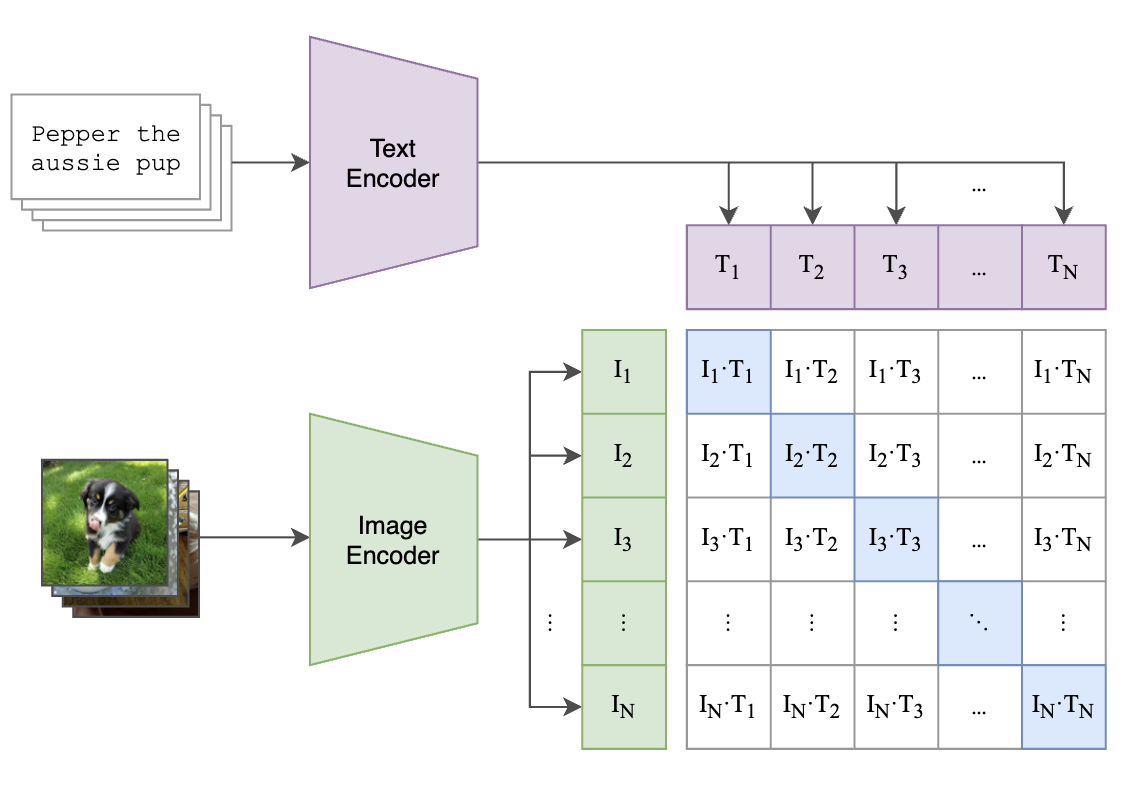
An image encoder extracts an embedding for each image in the batch. The text encoder does the same thing for the corresponding texts. They then use a contrastive loss to push matching image and text embeddings closer to each other, and repel pairs from different examples. The outputs from the encoders are first linearly projected into “multimodal embeddings”. We then take the cosine similarity of each pair of these image and text multimodal embeddings. Cross entropy loss is computed for each row (image-to-text) and column (text-to-image) of the similarity matrix. For each image we want to be able to predict the corresponding text, and vice versa.

The CLIP loss is a sum of two cross entropy losses. $\tau$ is the temperature, which is the exponentiation of a learned scalar $t$: $\tau = e^t$. The first cross entropy term is the image-to-text loss, which is minimized when the text embedding corresponding to an image has a high dot product with that image. The second term inverts this relationship to form a text-to-image loss.

\[\mathcal{L}_\text{CLIP} = \frac{1}{2n} \sum_{i=1}^{n} \left[ -\log \frac{e^{\tau \cdot I_e^{(i)} \cdot T_e^{(i)}}}{\sum_{j=1}^{n} e^{\tau \cdot I_e^{(i)} \cdot T_e^{(j)}}} \;-\; \log \frac{e^{\tau \cdot T_e^{(i)} \cdot I_e^{(i)}}}{\sum_{j=1}^{n} e^{\tau \cdot T_e^{(i)} \cdot I_e^{(j)}}} \right]\]

CLIP uses separate image and text encoders to map both into a shared embedding space for similarity comparison. Although the main goal of CLIP is representation learning, the resulting encoders can be used for zero shot tasks. You can specify many computer vision tasks as selecting a text among a group. For example, this can be applied to image classification. You can input a batch of images to the model. Rather than their corresponding captions, you input the classes as texts. The CLIP model can then match images to these arbitrary classes without any finetuning. Because it is trained on a large amount of images and text, this approach generalizes well.

The accuracy of the zero shot tasks can depend on how the texts are generated. Prompt engineering the class texts can improve performance. Multiple text prompts can be ensembled by averaging their embeddings.”

CLIP can also be used in a few shot setting by training a linear probe. This is just a single linear layer on top of the image encoder.

\[\text{logits} = W x + b\]

One clever trick is that the text embeddings can be used to warmstart a linear probe. Comparison with a set of text embeddings is mathematically the same as multiplying with a matrix containing the same number of rows.

\[W = \left[ w_1^{\text{zero-shot}},\ w_2^{\text{zero-shot}},\ \dots,\ w_C^{\text{zero-shot}} \right]^\top\]

Jia et al. 2021 released ALIGN shortly after which implements a similar approach. This method uses a different model architecture but uses the same contrastive training method. The dataset is much larger but noisier.

SigLIP

SigLIP, introduced by Zhai et al. 2023, replaces the softmax-based contrastive learning approach used in CLIP with a pairwise sigmoid loss. Instead of computing softmax across all pairs in a batch, SigLIP treats each image-text pair as an independent binary classification problem. This makes the training easier to parallelize across the batch.

\[\mathcal{L}_{\text{SigLIP}}= -\frac{1}{N} \sum_{i=1}^{N} \sum_{j=1}^{N} \log \frac{1}{1 + e^{z_{ij} (-\tau \cdot I_e^{(i)} \cdot T_e^{(j)} + b)}}\]

The loss is computed for each image and text pair independently. Since most of the $N^2$ pairs are not matching, a learnable bias $b$ is used to correct this.

The advantage of this compared to CLIP is that we do not need to calculate a global normalization factor for the cross entropy. The SigLIP loss can be better parallelized across devices.

Each device gets a chunk of the images. In step 1, they compute the loss with respect to the matching chunk of text. Each device then iterates through the other chunks of text embeddings (containing only negatives) and accumulates the loss.

CapPa

An alternative to the contrastive training methods of CLIP/ALIGN and SigLIP is image captioning. The pretraining task is to predict the text from the image. This is also closer to how the vision encoder will be used in a VLM.

Captioning is an alternative training method. A transformer decoder (LLM) is trained to predict the text, while attending to the image through cross attention. This contrasts with contrastive approaches in that we are generating the text, rather than text embeddings. This requires a decoder architecture for the text encoder.

In addition to captioning (Cap), this work also incorporates parallel decoding to get CapPa. Instead of auto-regressive token prediction, the model predicts all tokens simultaneously. This is done by masking out all of the input tokens to the model and replacing causal attention with bidirectional self attention. The model switches between these autoregressive and parallel decoding modes. The authors find that this mixture performs better than using either mode alone.

CoCa

This paper introduces Contrastive Captioner (CoCa), which is a method that unifies the contrastive and captioning approaches to learning from image text pairs.

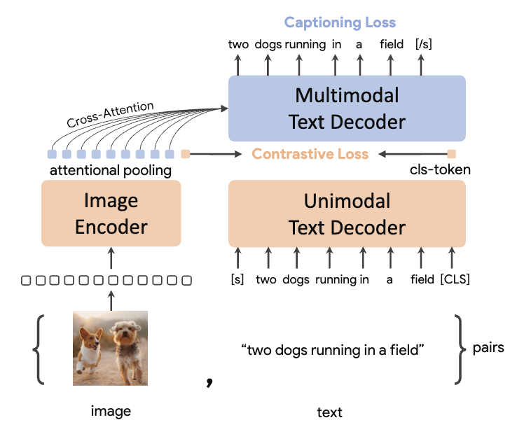
CoCa combines both approaches by training with a multi-task loss function that incorporates both contrastive learning and captioning objectives. Unlike CapPa, CoCa’s text decoder is split into unimodal and multimodal components.

The loss is a weighted combination of contrastive and captioning losses:

\[\mathcal{L}_{\text{CoCa}} = \lambda_{\text{Con}} \cdot \mathcal{L}_{\text{Con}} + \lambda_{\text{Cap}} \cdot \mathcal{L}_{\text{Cap}}\]

Attention pooling aggregates the vision embeddings into a single embedding, which is paired with the text decoder’s CLS token embedding for the contrastive loss. This implements a CLIP-style loss. A separate attention pooling layer creates embeddings for the multimodal text decoder. The decoder then uses standard next-token prediction loss for caption generation.

The contrastive loss can suffer from the hard negatives problem, where random sampling doesn’t yield the hard negatives that the model needs to learn fine-grained distinctions. The challenge with captioning is that it forces the model to predict very specific details that may be noisy or inconsistent across large datasets, making it overly sensitive to fine-grained variations that parallel the hard negatives issue. Combining these losses is a promising approach to get the best of both worlds.

Dynamic Resolution

So far, we’ve discussed encoders that process fixed-resolution images, such as 224×224 or 384×384 pixels. However, this approach has fundamental limitations. High-resolution images lose important details when downscaled, while low-resolution images waste computational resources when upscaled with padding. Unlike CNNs, transformers can handle variable-sized inputs—a capability we should leverage for vision tasks.

Modern VLMs have shifted toward dynamic resolution approaches that can handle variable input sizes more effectively. Rather than forcing all images into the same resolution, these methods adapt the processing to match the image’s native aspect ratio and information density. Implementation approaches include Native Resolution ViT and dynamic tiling, though we won’t cover these in detail here.

VLM Architectures

In multimodal ML and data processing, there are different ways to combine modalities:

• Early fusion: Combine modalities at the input level, processing them together through the entire model
• Late fusion: Process each modality separately and combine their outputs at the end
• Middle fusion: Combine the modalities at an intermediate representation

For modern VLMs, the general pattern is to use vision encoders for additional processing of visual data. LLMs prioritize language, with most of the training focused on language. Visual data is processed and adapted specifically for use by the language model.

Late fusion wouldn’t be effective for VLMs since the LLM needs access to visual data earlier in the pipeline to generate appropriate text outputs.

Intermediate fusion, where vision embeddings are added at a middle layer, could potentially lower computational costs. Visual data adds many embeddings and increases context length significantly. By skipping earlier layers, we could reduce computation and shrink the KV cache size. However, this approach isn’t commonly implemented in state-of-the-art VLMs, as model quality is generally prioritized over efficiency.

Early fusion VLM architectures use a vision encoder to output a sequence of vision embeddings. These embeddings are processed by an adapter before being appended to the LLM’s input. Typically, the LLM applies full attention to these visual tokens while using causal attention for the language tokens. This approach works because the model isn’t generating the image tokens but using them to generate text. Models that perform autoregressive image generation are an exception to this pattern (it’s rumored that GPT-4o uses this approach). Chameleon from Meta implements this. Currently, it is more popular to have separate models for image generation, so we’ll focus more on images as inputs rather than outputs.

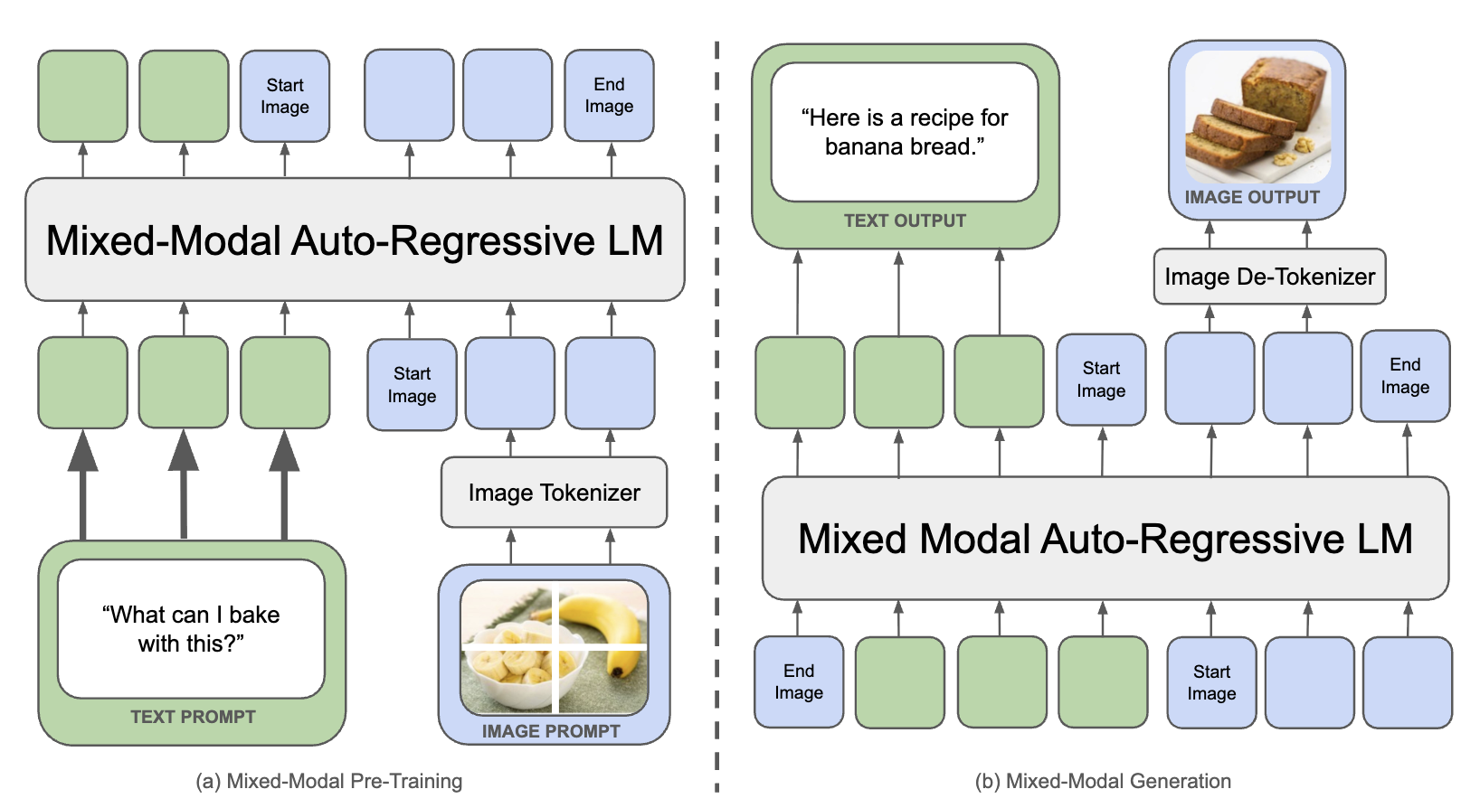
Transformers have a quadratic computational complexity with respect to token length. Images introduce a large number of tokens, particularly at high resolutions, significantly increasing the computational demands on the LLM. When designing VLM architectures, token compression becomes essential. Several techniques exist to reduce the number of visual tokens that the language model must process.

We will now examine the architectural patterns used in VLMs. For early fusion, there are two main approaches: inserting vision tokens into the input sequence with an MLP adapter, or using cross attention with learned query embeddings.

Cross Attention Adapter

Cross attention adapters, also called attention poolers, compress sets of embeddings into a fixed number of output embeddings using learned query embeddings. These learned query embeddings attend to the vision tokens through cross attention, where keys and values are derived from the vision encoder’s output.

This is implemented in Qwen-VL as a “position-aware vision-language adapter”. The number of query embeddings dictates how many embeddings we choose to represent the image. There is a trade-off between capturing more information and reducing the sequence length that the LLM sees.

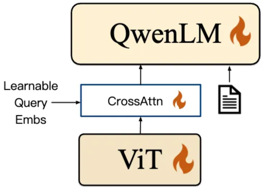
This cross attention layer is added in between the ViT and the LLM. The existing transformer blocks of the vision encoder and language model are not modified.

This architecture can gracefully handle different resolutions of images, but they train with 224x224 and post-train with 448x448. For the higher resolution post training, they increase the number of query embeddings from 256 to 1024.

MLP Adapter

In the LLaVA work by Liu et al. 2023, the authors train a simple VLM architecture by combining a pretrained LLM (Vicuna model, open-source instruction-tuned LLaMA) and a pretrained vision encoder (CLIP ViT-L). The vision tokens are linearly projected and then concatenated to the input of the LLM decoder.

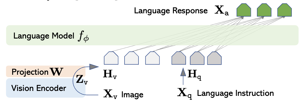
This approach is currently more popular than cross attention. Qwen switched to MLP for Qwen-VL2. LLaMA 3.2-Vision, PaliGemma 2, and DeepSeek-VL also use MLP adapters.

With MLPs, we have less control over the token lengths. The simplest way to compress the token length is to project multiple vision encoder embeddings into the same input embedding. This is used in Qwen2.5-VL. Groups of 4 vision tokens are concatenated and passed to a two-layer MLP. This projects each group to a single embedding of the LLM’s dimension.

BLIP

BLIP-2 (Li et al. 2023) uses a Querying Transformer or Q-Former as an adapter. These architectures are similar to Flamingo in that they keep the vision encoder and text decoder frozen. However, BLIP is actually an early fusion architecture.

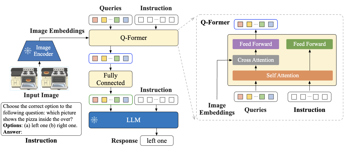
The Q-Former is similar to the Perceiver in that it processes images with a fixed number of learned query embeddings. However, it also takes in the text tokens. The text input shares the self attention layer but skips the vision cross attention and learns a new feed forward layer.

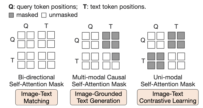
This is trained in two stages. In stage 1, three losses are optimized: Image-Text Matching (ITM, binary classification of whether image-text pairs match), Image-Grounded Text Generation (ITG, next token prediction loss conditioned on image), and Image-Text Contrastive Learning (ITC, CLIP loss). These different losses are set up by changing the attention masks.

In Stage 2, they connect the Q-Former to a frozen LLM, by concatenating the visual outputs to the LLM’s inputs. The text component of the Q-Former is discarded. This is finetuned to generate text.

Cross Attention Mid Fusion

The cross attention adapter uses attention to map embeddings to the input of the language model. An alternative design would be to add cross attention to the transformer blocks of the language model. These methods aren’t as popular as early fusion but are worth exploring.

Flamingo

Alayrac et al. 2022 introduce the Flamingo VLM architecture. It keeps the vision encoder and LLM parameters frozen but adds perceiver resamplers and gated cross-attention dense blocks. Since the LLM parameters are frozen, this method has no effect on the text only performance of the model and we can easily recover the text only LLM by deleting these additional modules.

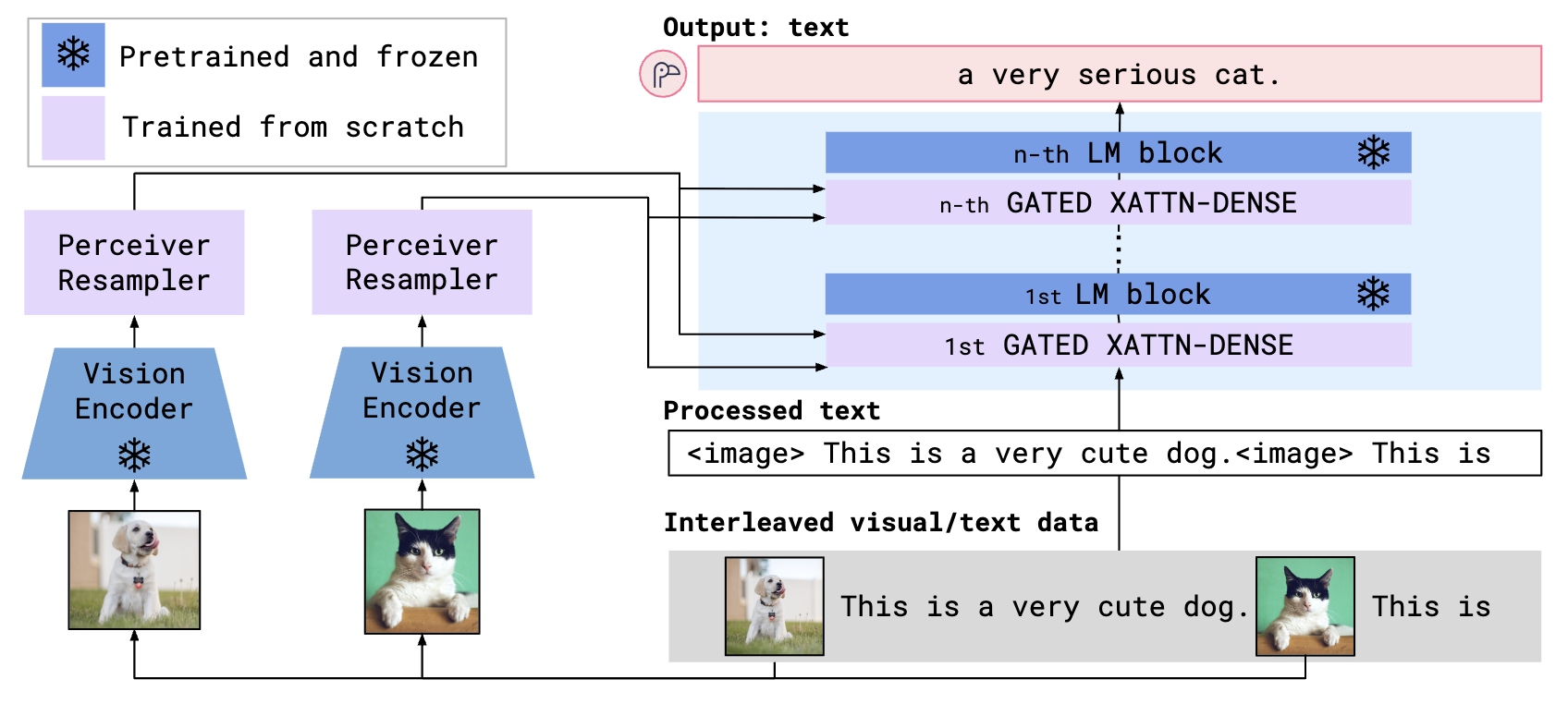
The perceiver resampler takes a variable number of input embeddings and outputs a fixed number of output embeddings. It is essentially an attention pooler with a feed forward layer that is repeated by num_layers.

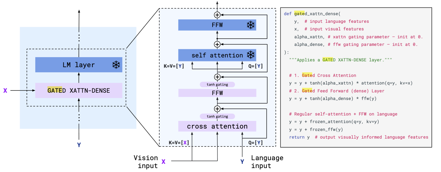
The gated cross attention dense layers are similar to the cross attention layers in encoder-decoder transformers. It is gated by layer specific learnable alpha parameters. These are initialized to 0, so the added vision modules have no impact at the start of training. The tanh activation ensures non-zero gradients for the alpha parameters after initialization.

While architecturally interesting, Flamingo’s approach has been superseded by simpler early fusion methods in modern VLMs. Generally, we don’t want to separate the vision and language parameters of our models. We want foundation models that are natively multimodal.

LLaMA

LLaMA 3.2 uses a ViT encoder trained with a contrastive objective for visual understanding. However, they discovered that the contrastive objective doesn’t preserve fine-grained localization information. To address this, they extract features from multiple layers (4th, 8th, 16th, 24th, and 31st) of the encoder.

They enhance the encoder by adding 8 additional transformer layers. The original ViT encoder, trained with CLIP, has 32 layers. These 8 extra layers increase the total to 40 and are designed to learn features more relevant to language generation. Both the attention and feed-forward layers in these additional layers use tanh gating. Unlike Flamingo, the gating parameters are initialized to $\pi/4$ instead of 0 (code), which effectively reduces the contribution of these added layers by about 40%.

The language decoder incorporates cross attention for images in every fourth transformer block. Unlike Flamingo, LLaMA doesn’t gate this cross attention.

LLaMA 3’s architecture is distinctive for using a mid fusion approach, setting it apart from most other models. This approach was necessary because LLaMA 3 was originally developed as a text-only model, and mid fusion is often required when adapting text-only models to handle images. However, with LLaMA 4, Meta transitioned to an early fusion MLP adapter approach, which they market as “native multimodality.” For early fusion to work effectively, the model must be trained end-to-end from early in the training process.

Training Recipes

LLMs undergo training through a progressive multistep pipeline. For text-only LLMs, we usually have the following stages: pretraining → supervised fine-tuning (SFT) → reinforcement learning (RL). Let’s examine how visual capabilities are integrated into these training pipelines.

LLaVA

The training recipe of LLaVA has two stages. The first stage involves pretraining the model on 595k image-text pairs filtered from the CC3M image pair dataset. The goal is to align visual and language representations. Only the MLP projector is unfrozen in this stage. The model is prompted to generate a brief description of the image, with a randomly sampled question (ex: “Summarize the visual content of the image.”, Appendix E). This prompt is generic and doesn’t consider the content of the image-text pair, however at this stage we only need to train the adapter.

In stage 2, the LLM and projector are unfrozen while the vision encoder stays frozen. The model is finetuned on higher quality data and more complex prompts. At the time of release, multimodal instruction following data was scarce. The authors addressed this gap with a synthetic data strategy. They leveraged a language only GPT-4 model to generate diverse questions related to the image. Note that the image itself is not used in the generation of these prompts. Instead, they input the caption of the image as well as bounding boxes if available.

To guide GPT-4’s generation, the authors manually designed seed examples for three data types. Conversations create multi-turn dialogues with simple questions and answers about details in the image such as object types, counting, locations, and spatial relationships. Detailed descriptions generate comprehensive scene descriptions that describe each object in the image. Complex reasoning involves more complex questions that require multiple steps to arrive at an answer. These seed examples were the only human annotations needed and enabled GPT-4 to generate thousands of similar examples through in-context learning.

Qwen-VL

In the pretraining stage, both the vision encoder and the adapter are unfrozen. Qwen trains at a much larger scale than LLaVA, using 5 billion image-text pairs. They initially pretrain at a lower resolution and then switch to higher resolution images for subsequent stages.

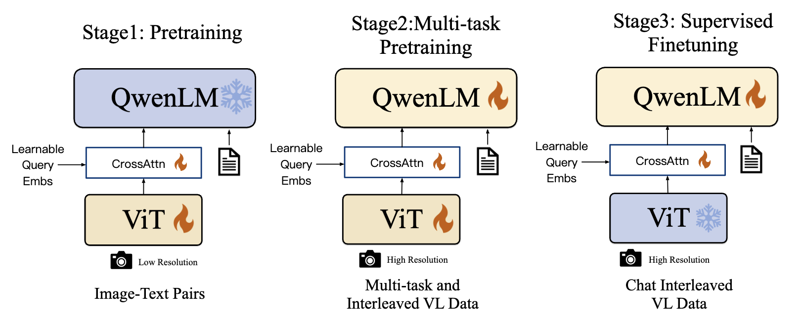
The multi-task training phase uses higher quality data covering various vision-language tasks, including captioning, visual question answering, grounding, and OCR. They also incorporate text-only data to maintain the model’s text generation abilities. All components remain unfrozen during this stage to develop general visual understanding, using 76.8 million examples.

In the final stage, the model is finetuned specifically for improved instruction following and dialogue capabilities. Since this stage doesn’t target better image understanding, the ViT is frozen. This phase uses a small but high-quality dataset of only 350k examples focused on multimodal instruction following and captioning. This progression demonstrates how each stage uses progressively less data of increasing quality.

Qwen2-VL uses the same training recipe but significantly scales up the datasets. It also uses the Native Resolution ViT architecture for dynamic resolution with the vision encoder. Unlike Qwen-VL, which used fixed image resolutions, Qwen2-VL also adds video support to both its architecture and training data.

Qwen2.5-VL further improves this training recipe by scaling up sequence length, which is crucial for handling longer videos. The first two training stages maintain the same sequence length. However, Qwen2.5-VL replaces stage 3 with “Long-Context Pretraining,” where the model is trained end-to-end (with both ViT and LLM unfrozen) on long-context data such as extended videos or images with substantial text. On top of these three pretraining stages, they add SFT and RLHF (DPO) post training stages.

They also show that this VLM training slightly reduces the text only performance of the LLM. This may be why VLMs are often released separately from the base text models.

DeepSeek-VL

The same pattern is used in DeepSeek-VL, except the vision encoder is not frozen during the SFT stage.

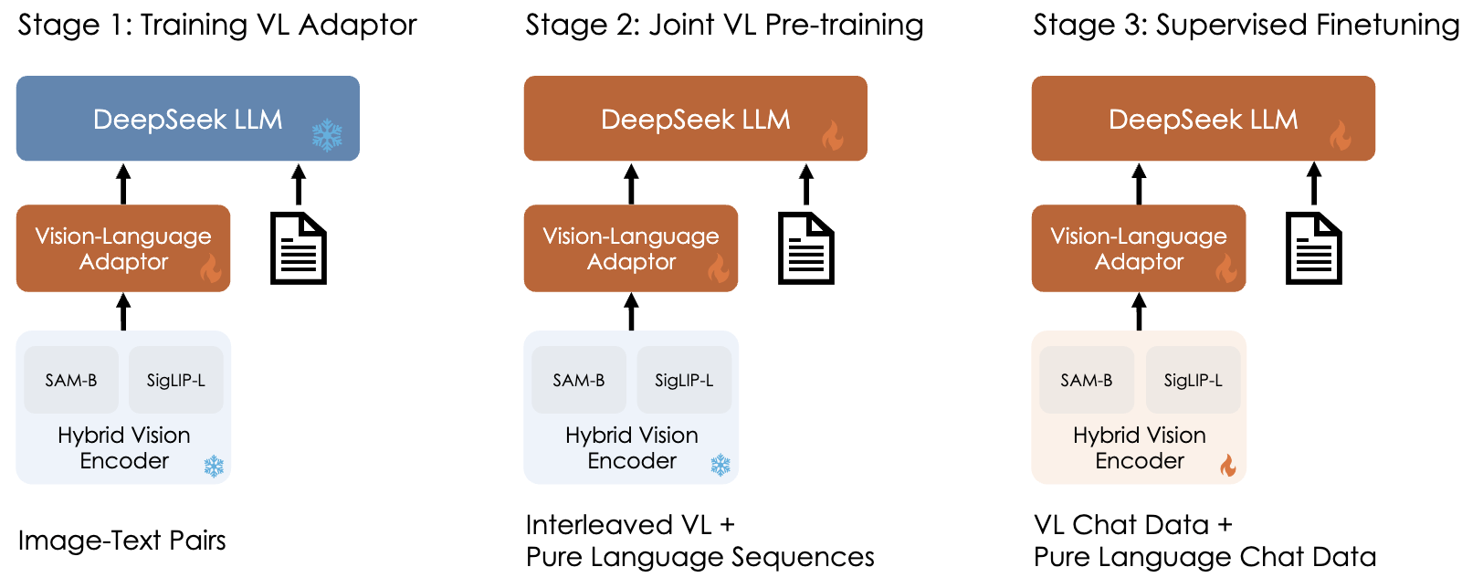
In DeepSeek-VL2, they introduce a dynamic tiling strategy to enable dynamic resolution. The same training stages are applied but with scaled up and improved datasets.

Kimi-VL

Kimi-VL follows a strategy similar to Qwen2.5-VL. They pretrain MoonVIT, a dynamic resolution vision encoder. Both the Qwen2.5-VL and Kimi-VL vision encoders are trained using SigLIP and captioning losses, similar to CoCa. Unlike approaches that freeze certain components, Kimi-VL trains all parameters during each stage.

During joint pretraining, the VLM trains on both image-text pairs and text-only data. This balanced approach is crucial at scale to prevent degradation of text generation capabilities. The cool down stage uses higher quality data, while the long context stage incorporates both long-context text and multimodal examples. A notable feature of Kimi’s approach is the inclusion of both text and multimodal inputs throughout all training stages. They continue training with SFT and RL post training stages to develop a multimodal reasoning model.

Despite variations in training pipelines, these models share common patterns. They all use multi-stage pretraining, with each progressive stage processing fewer examples but incorporating higher image resolution, longer context length, and improved data quality.

Video

We have focused on image inputs but VLMs can also be developed to understand video inputs. Rather than extracting tokens for a single image, you can process each frame separately and concatenate the tokens. Audio tokens can be processed separately and then interleaved/concatenated with the frame tokens.

One important thing to note is that video is far more expensive to process than images. A single image already requires hundreds to thousands of tokens, but videos add a high multiplier. For example, a 1-minute video at 30fps means processing 1,800 frames. Depending on the tokenizer, each frame could be 256 tokens. This means the one minute video would be 460k tokens. If we use the rule of thumb that a token is equal to 3/4 of a word, this means this is equal to 345K words. If we assume there are 500 words on a page, this is approximately equivalent to a 700 page book. However, a minute of video has far less useful information than a long book. This redundancy creates opportunities for compression, which is critical for processing longer videos.

The simplest way to reduce token count is to choose a low frequency to sample the video frames in order to reduce processing and token count. If we use 1 FPS, we reduce the token count for 1 minute of video to 15K tokens. It is impractical to train a VLM with videos at full frequency.

There are some interesting works on making this more efficient, leveraging the fact that there is a lot of redundant information between nearby video frames. One simple method is to project patches from multiple frames to a single token. Qwen2.5-VL does this through a strided Conv3D. Typically in a vision transformer encoder, the image is split into 2D patches which get projected to a token embedding (equivalent to a strided Conv2D). Qwen uses 3D patches. This aggregates information from multiple frames into individual tokens. This is like reducing the frame frequency while not dropping any frames entirely.

There are more sophisticated methods that allow for a more dynamic compression that takes into account the variable amount of redundancy. For example, Run-Length Tokenization (RLT) (Choudhury et al. 2024) identifies consecutive patches that are repeated across video frames and replaces them with a single token plus a duration encoding. Consecutive patches are considered repeated if the L1 distance between them is below a threshold $\tau$. This method is content-aware in that the number of tokens depends on how redundant the frames of the video are.

RLT is a simple heuristic-based method of video token compression. There are also model based approaches for this.

Conclusion

When I first started working on ML, it seemed like computer vision and natural language processing were parallel and equally important fields. There was some knowledge transfer, but they were fairly independent, both in training methods and model architectures. Transformers were invented for NLP but were soon applied to other data modalities including vision. More recently, LLMs have been dominating the field of AI. As these models have become more multimodal, it seems like other domains are getting absorbed into LLM research. While computer vision remains an active area of research, a large portion of the field is focused on improving the visual capabilities of LLMs.

This convergence and the rise of VLMs is leading to many interesting applications, such as action planning in robotics and visual accessibility tools. As these models continue to improve, we’re moving closer to AI systems that can understand the real world, which is very visual.