A crucial aspect of both human and animal intelligence is our internal model of the world. We use this model to predict how our actions will affect our environment, anticipate future events, and plan complex sequences of actions to achieve goals. Most current machine learning research focuses on models that passively understand data, like image classifiers or captioning models. However, to create AI systems that can truly interact with their environment rather than just observe it, we need effective world models that learn how actions influence the environment.

It is a common objective for machine learning models to predict future observations based on current and past observations. Language models, for instance, predict subsequent words from preceding ones. World models extend this concept by incorporating actions. These models learn how actions affect the environment, enabling the development of intelligent agents that can effectively plan and interact with their surroundings.

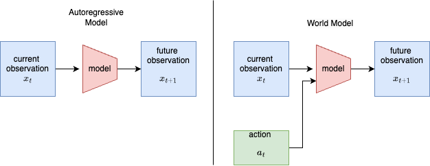
A world model is a function that maps the current state of the world \(x_t\) and an action \(a_t\) to a prediction of the next state \(x_{t+1}\). The definition of observation and action varies depending on the implementation.

World models enable many important capabilities for intelligent systems. Learning an effective world model requires understanding physics, causality, spatial intelligence, and more. These are especially important as we deploy AI systems in the real world.

World models have diverse applications across different domains. While significant research has focused on video game environments for training game-playing agents, their most crucial application lies in real-world embodied AI. Robotics applications require world models to understand and interact with their physical environment, predict the outcomes of their actions, and adapt to changing conditions. These models help robots perform complex tasks that require planning.

World models represent an exciting but still nascent area of AI research. The term “world model” remains somewhat loosely defined. In this blog post, we will discuss different implementations of world models.

Generative World Models

World models have immediate applications in physical AI, particularly in robotics and autonomous vehicles. These systems require interactive data that demonstrates how actions lead to specific outcomes, unlike traditional vision models that simply observe static data.

A significant challenge in robotics is the limited availability of training data compared to language models. While the most valuable data comes from real-world interactions with physical agents, collecting this data is both expensive and time-consuming. We also need a large amount and variety of environments so the agents can learn to generalize well. The goal of this class of world models is to generate realistic and diverse environments in order to train robust agents.

Genie

This work from Google is a “generative interactive environment” trained on internet data (Genie-2 Blog Post). It is capable of generating interactive environments from a text or image prompt. We will explain each component of the model.

Spatial-Temporal Transformer

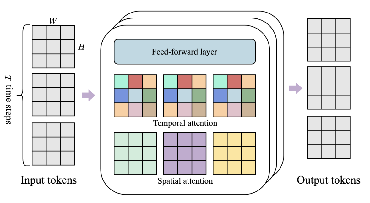
Since it is trained on videos, Genie uses the Spatial-Temporal Transformer (ST-Transformer) architecture to implement most model components. The ST-Transformer block has three components, temporal attention, spatial attention, and a single feed forward block. The spatial attention is self attention among patches of a single frame. The temporal attention is for a single patch on \(T\) time steps. This uses causal attention. This architecture scales linearly rather than quadratically with the number of frames, which makes it efficient at processing video.

Latent Action Model (LAM)

In world models, we need to associate actions with transitions between observations. Since actions are not available on internet scale data, this model learns “latent actions”. This model uses an encoder and decoder. The input to the encoder is all prior frames \(x_{1:t}\) and the next frame \(x_{t+1}\). The encoder outputs latent actions \(\tilde{a}_{1:t}\). The decoder uses these latent actions and the prior frames to predict the next frame \(\hat{x}_{t+1}\). This is implemented using a VQ-VAE objective. A small code book of size 8 is used for controllability. The small codebook size also acts as a bottleneck. This forces the representation to only store information about the change rather than encode the observation itself.

When trained on 2d videos, the changes between frames can be described in a compact code. Think of moving left, right, jump etc. this may be more difficult in complex real world environments. Since the latent actions use a small codebook and the decoder has access to the prior frames, the model is forced to learn the differences between frames which can be represented as actions.

Video Tokenizer

Another VQ-VAE is trained to generate tokens from the video. The difference here is that the input and output are identical and just the video frames.

Dynamics Model

The dynamics model takes the prior video tokens and latent actions and predicts future video tokens. This also uses a ST-Transformer architecture. Since this is a causal transformer, at each timestep \(i\) the model uses the current latent embedding \(z_i\) to predict the next timestep’s embeddings \(z_{i+1}\). At training time, this is parallelized so \(z_{1:t-1}\) is mapped to \(z_{2:t}\).

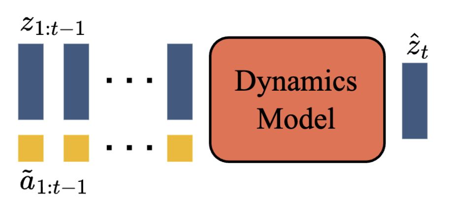
The MaskGIT method enhances this model’s performance. Since we’re dealing with images/video frames, \(z_i\) represents a grid of latent embeddings. Traditional autoregressive prediction of these embeddings in one shot can be unstable. In this setting, if a single token is mispredicted, all subsequent predictions suffer. MaskGIT resolves this through an iterative process that enables prediction corrections. The tokens within the next frame can attend to each other bidirectionally.

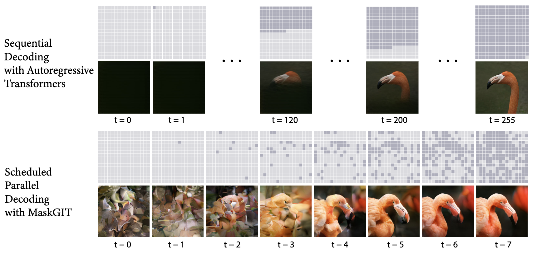
During training, tokens are randomly masked according to a Bernoulli distribution with a sampled probability between 0.5 and 1, and the model predicts these masked tokens. This training approach enables iterative decoding at inference time. The next frame is initialized as zeros, and the dynamics model makes predictions based on the context. The dynamics model then processes this output as an input. Since the predictions are a softmax over discrete token values, we can determine which tokens are low in confidence. The model in subsequent iteration only updates these low confidence predictions. This is repeated across 25 steps, where output tokens are regenerated until reaching high confidence. This method is similar to diffusion, but uses discrete rather than continuous tokens. The masking approach makes the dynamics model’s predictions more robust and reduces the redundancy in video data for more efficient learning.

Training and Inference

The latent action model and video tokenizer are trained separately first. They are trained using the VQ-VAE objective. The LAM and video tokenizer are then used to train the dynamics model. There is a stop grad so that the latent action model is frozen.

At inference time, the LAM is discarded as we can define the actions directly. The model is prompted with a single initial frame which is tokenized. At each step, the user chooses an integer for the latent action. The initial frame tokens and the latent action are used to generate the next latent token. This generated token is appended to the input . The user can then select another action. At each step, the tokenizer decoder can map the latent embeddings to images which can be displayed to the user.

The video tokenizer and LAM are very similar. One significant difference is that LAMs use smaller codebook sizes. The focus is on having a controllable set of actions (8 codes). The video tokenizer uses a larger codebook size (1024) to more effectively reconstruct the video. The LAM is able to use a smaller codebook size since it is only trying to encode one frame at a time. Whereas the video tokenizer tokenizes the entire video and then reconstructs it all together.

---

Genie achieves a significant breakthrough by training on large-scale data without requiring explicit actions. Instead, it learns a finite set of latent actions that enable interaction with generated environments.

Through these latent actions, users can control newly generated games. While this approach is powerful because it enables training on extensive datasets without ground truth actions, the learned actions come with limitations. Since the actions are discovered rather than defined, there’s no way to enforce specific mappings. For example, with 4 latent actions, we cannot guarantee that action 1 means “move left” and action 2 means “move right.” The model might learn diagonal movements instead. This use of latent actions somewhat weakens Genie’s classification as a true world model, since traditional world models aim to learn how observations change based on well-defined, real-world actions.

Cosmos

Released by NVIDIA, Cosmos is a “world foundation model”. It is trained on a large dataset of 20 million hours of video. Unlike other works, Cosmos focuses on physical AI and real world data rather than simulated video game environments. It is built for physical AI applications like robotics and autonomous vehicles. We will cover the different components of this model.

Tokenizer

Effective world modeling requires efficiently tokenizing videos. They make available both discrete and continuous tokenizers. They are both trained in the same way, but the discrete tokenizer uses Finite-Scalar-Quantization (FSQ) to discretize the tokens.

The tokenizer models use a temporally causal encoder-decoder architecture to map videos from \(x_{0:T} \in \mathbb{R}^{(1+T) \times H \times W \times 3}\) to “token videos” \(z_{0:T'} \in \mathbb{R}^{(1+T') \times H' \times W' \times C}\) which are more compact spatially and temporally. To train this, they use a simple L1 reconstruction loss. In a second stage of training, they use an optical flow loss to improve the smoothness between frames of the video, and a Gram-matrix loss to improve the sharpness of the frames. An adversarial loss is used to further enhance this.

World Model

Like with tokenizers, the world model is also implemented for continuous and discrete tokens. However, the model architectures are more different. Diffusion is used for continuous tokens, while autoregressive models are learned with the discrete tokens.

Diffusion

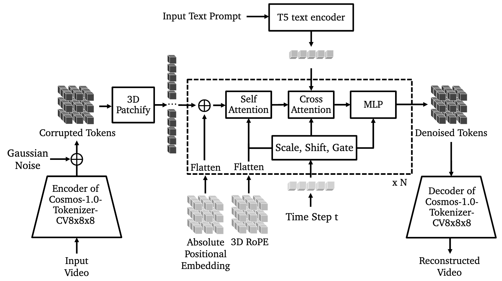
They use a DiT (Diffusion Transformer) based architecture. The continuous tokens are perturbed with Gaussian noise and the DiT model denoises these tokens. The model is conditioned on text through cross attention. The text prompt provides additional information about the video that is used for denoising. At inference time, the text can be used to generate new videos. The model can also be conditioned with input image frames to generate video continuations.

Autoregressive

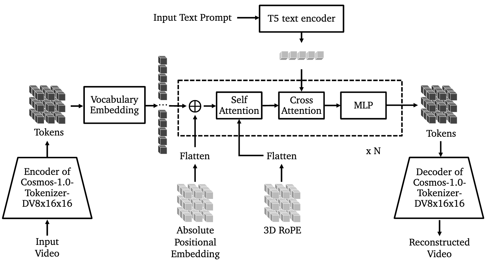
The autoregressive world model trains on the next token prediction objective using discrete video tokens. This training happens in multiple stages:

Stage 1: Predict tokens of future frames given a context of the first 17 frames.

Stage 1.1: Context length is increased to 34 frames. Note that each frame produces a large number of tokens.

Stage 2: Train with text conditioning.

A diffusion model is used as a decoder to achieve higher quality video generations. This decoder is trained separately.

---

Cosmos includes two other classifications of world models. Text2World maps text prompts to videos. Video2World models take text prompts and video as input. These models generate continuations of the video.

In Cosmos, actions are referred to as perturbations or \(c_t\). During WFM training, these perturbations are simply text prompts describing the videos. Text effectively encodes actions when continuing videos, allowing for generalizable world model training. During finetuning, actions can be encoded in more specific formats. For example, when finetuning on camera control, the model is conditioned with Plücker coordinates that represent the camera’s pose. The model learns to generate video matching these coordinates. Additional models can also be incorporated to condition the WFM on task-specific actions.

During world model pretraining, explicit actions aren’t used. The model functions essentially as a video generation model. However, the models are later finetuned to incorporate explicit actions for different use cases, transforming them into true world models.

Cosmos was released very recently. It will be interesting to see whether “World Foundation Models” become more widely developed and used in the coming months. No model has been trained yet on this scale of physical AI data.

World Models for Agents

The previous works focus on generating interactive environments that can be used to train intelligent autonomous agents. Now, we will explore approaches that use world models to develop the agents themselves. This is essential for leveraging all the generated environments. We want to create autonomous agents capable of performing well across diverse environments and tasks, especially with limited data. World models provide valuable solutions to this challenge.

World models are an important component of model-based reinforcement learning. In MBRL, a dynamics model predicts the next state from the current state and action. There are different methods to use this for planning. Typically, the dynamics model is learned from a dataset of trajectories for the task at hand, from the real world or simulation. The states that are being predicted are task specific representations.

The dynamics model can be implemented with a world model. This is when the model is trained on a large and diverse dataset of offline data, rather than task-specific trajectories. World models enable learning a single dynamics model, which can generalize to multiple tasks. This is important for robotics, since you want the robot to be able to do things that aren’t optimized for during training. For this generalization, it is important that the world model is trained on a variety of tasks so it doesn’t focus on task-specific information.

Ha et al. 2018

This relatively early paper shows the advantages of world models in the context of reinforcement learning. They train world models on different OpenAI Gym environments to learn effective policies.

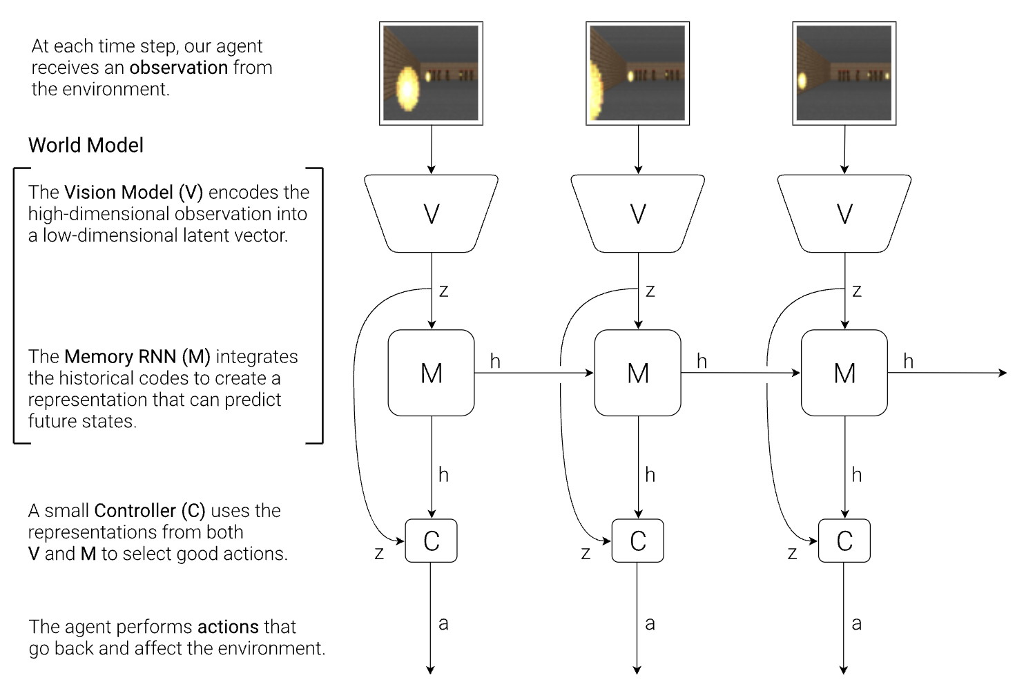
V: The vision model is a VAE that learns a latent representation \(z\) of the observation (image) from the environment.

M: The memory RNN learns representations across time and makes predictions in the latent space. It is modeling \(P(z_{t+1}\mid a_t, z_t, h_t)\). The next latent representation is predicted from the current representation, action, and hidden state. This is a probability distribution using a mixture density model, so we can sample from it.

C: The controller predicts an action from the hidden state and current latent representation. This can be a lightweight linear model.

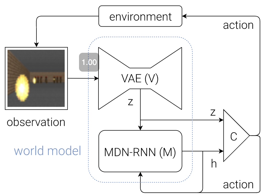
Steps to train

1. Generate rollouts under a random policy
2. Train \(V\)on the frames
3. Train \(M\) on the latent representations and the actions of the random policy
4. Optimize the controller
5. Restart to learn from rollouts from the new policy

We can also use the world model to generate new rollouts in the latent space. This is done by sampling latent representations in \(M\) and using it to train the controller. One issue with this approach is that the policy can exploit gaps in the world model. The stochasticity of \(M\) helps train a more robust controller.

This early work laid important foundations for subsequent research in world models, showcasing their potential for creating more sample-efficient and generalized learning systems.

Dreamer

The paper “Mastering Diverse Domains through World Models” by Hafner et al. 2023 introduces the DreamerV3 model. This line of work aims to train world models to use for model-based reinforcement learning. This approach utilizes two stages: world model learning and actor critic learning.

World Model

The world model is implemented as a Recurrent State-Space Model (RSSM), which is learned using trajectories with frames and actions.

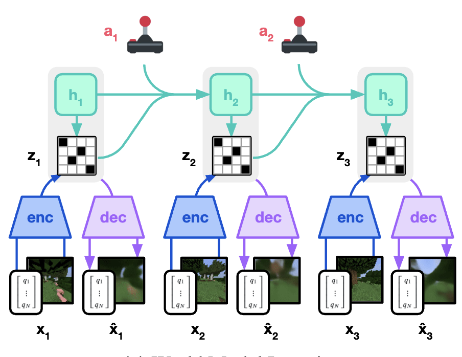
Sequence model \(h_t=f_{\phi}(h_{t-1},z_{t-1},a_{t-1})\): This model predicts the next hidden state from the prior hidden state, latent representation, and action.

Encoder \(z_t \sim q_{\phi}(z_t \mid h_t, x_t)\): This model generates the latent representation of a timestep \(z_t\) from the observations (frames). This also utilizes the hidden state \(h_t\).

Dynamics predictor \(\hat{z}_t \sim p_{\phi}(\hat{z}_t\mid h_t)\): This predicts the latent representation from the hidden state.

Reward / Continue predictor \(\hat{r}_t \sim p_{\phi}(\hat{r}_t \mid h_t, z_t)\), \(\hat{c}_t \sim p_{\phi}(\hat{c}_t \mid h_t, z_t)\): These models predict the reward and continue signal. The RL environments are set up to have a scalar value for these at each timestep.

Decoder \(x_t \sim p_{\phi}(\hat{x}_t \mid h_t, z_t)\): This predicts the observation frame from the latent representation. The decoder is not necessary for planning but training with it ensures that \(z_t\) captures information from the observations. This model also enables visualizing planned trajectories. The encoder and decoder together form a discrete autoencoder.

---

With these modules, we can train the world model using offline trajectories. There are three different losses which train different modules.

\[\begin{aligned} L_{\text{pred}}(\phi) &= -\ln p_{\phi}(x_t \mid z_t, h_t) - \ln p_{\phi}(r_t \mid z_t, h_t) - \ln p_{\phi}(c_t \mid z_t, h_t) \\ L_{\text{dyn}}(\phi) &= \max(1, \text{KL} [\text{sg}(q_{\phi} (z_t \mid h_t, x_t)) \mid\mid p_{\phi}(z_t \mid h_t)]) \\ L_{\text{rep}}(\phi) &= \max(1, \text{KL} [ q_{\phi}(z_t \mid h_t, x_t) \mid\mid \text{sg}(p_{\phi}(z_t \mid h_t))]) \end{aligned}\]

The prediction loss \(L_{\text{pred}}\) trains the decoder, reward predictor, and continue predictor (corresponding to the three terms in the equation). \(L_{\text{dyn}}\) and \(L_{\text{rep}}\) train the encoder and dynamics model, similar to the VQ-VAE codebook and commitment losses (VAE blog). The dynamics loss trains the dynamics predictor to predict latent representations from hidden states that match the encoder’s output, while the representation loss trains the encoder to generate latent representations that match the dynamics predictor’s output. These losses are clipped so the learning focuses on the prediction loss when the other two are reasonably optimized. This also prevents the encoder from including irrelevant information in the representations, which makes control more difficult. The sequence model isn’t directly included in any of these losses, but receives gradients as we generate hidden states through the trajectories.

These losses are weighted and calculated for each timestep of the trajectories to train all the modules of the world model at once.

\[\mathcal{L}(\phi) \doteq E_{q_{\phi}} \left[ \sum_{t=1}^{T} \left( \beta_{\text{pred}} \mathcal{L}_{\text{pred}}(\phi) + \beta_{\text{dyn}} \mathcal{L}_{\text{dyn}}(\phi) + \beta_{\text{rep}} \mathcal{L}_{\text{rep}}(\phi) \right) \right]\]

Actor Critic Learning

Once we train the world model using offline trajectories, we can use actor-critic learning on simulated online trajectories. This is a popular RL method. The actor (\(a_t\sim \pi_{\theta}(a_t\mid s_t)\)) predicts the action to take given the current state. The critic (\(v_{\psi}(R_t\mid s_t)\)) predicts the expected sum of future rewards for a state.

Rather than interacting with real environments, the actor can be trained on imagined trajectories from the world model. The world model and actor simulate trajectories along with reward and continue signals. This stage is the dreaming. The critic is trained to learn the sum of rewards, while the actor learns a policy to maximize returns. This enables learning an effective policy with simulated interactions.

The actor and critic are trained concurrently on both imagined trajectories from the world model and real trajectories stored in a replay buffer. While the world model improves sample efficiency, some real interaction is still needed to fine-tune on the specific task. The ratio of imagined to real trajectories and the weighting of losses are tunable hyperparameters.

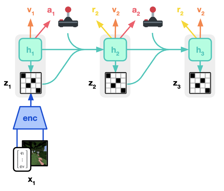
Dreamer uses a general purpose world model to be able to more effectively and efficiently learn policies for a variety of tasks and environments. One shortcoming of Ha et al. 2018 and Dreamer is that they only use trajectories with rewards for training. As we know, this kind of data is limited. We want to be able to train with videos that have no actions and rewards, and even with static unlabeled images.

DINO-WM

This method uses a pretrained DINOv2 SSL model (covered here) to bootstrap a world model. The DINO model is trained at a very large scale to produce image representations for visual understanding. This method incorporates this capability as a component of a world model, rather than trying to learn it through the world model itself.

The authors also opt for avoiding reconstruction of images and rather predict latent representations. This follows the JEPA framework.

The environment is modeled as a partially observed Markov Decision Process POMDP defined as \((\mathcal{O},\mathcal{A},p)\) (observations, actions, probability). Like the other methods, there are three components of this world model:

\[\begin{aligned}\text{Observation model} &: z_t \sim \text{enc}_\theta(z_t \mid o_t) \\\text{Transition model} &: z_{t+1} \sim p_\theta(z_{t+1} \mid z_{t-H:t}, a_{t-H:t}) \\\text{Decoder model} &: \hat{o}_t \sim q_\theta(o_t \mid z_t)\end{aligned}\]

The observation model learns a latent representation. The transition model predicts future representations given the prior observations and actions. The decoder model reconstructs the image observation, which is optional (visualization/generation).

Observation Model

The observation model is trained to learn visual representations. This model is meant to generalize to many tasks and environments. For this they use a pre-trained DINOv2 model. This model is trained on internet scale image data, so it generalizes well. At time step \(t\) it encodes an image \(o_t\) into patch embeddings \(z_t\) of shape \((N, E)\), where \(N\) is the number of patches and \(E\) is the embedding dimension.

Transition Model

The transition model is trained as a decoder-only transformer model. Given past latents, the model predicts future latents. Through an attention mask, patch embeddings indexed by \(i\) only attend to embeddings of the same index. That is the latent state \(z_t^i\) attends to \(\{z_{t-H:t-1}^i)_{i=1}^N\). \(H\) represents the context length, which is the number of steps the model can look back. There is attention between the patches in the observation model, but the transition model looks at each patch independently.

To incorporate actions, a K-dimensional vector is concatenated to each patch embedding in the input. This is mapped from the original action representation, which is a continuous vector defining the action, using an MLP. The representation of an action changes based on the environment or task. For example, it could be a 2D vector like (-0.1, 2.1), describing how to push an object. The actions are included in the training datasets. This model is trained with teacher forcing using these trajectories.

Additional metadata, such as proprioceptive information, can also be mapped to embeddings and concatenated. The model is trained with a simple L2 loss:

\[\mathcal{L}_{pred} = \left\| p_\theta \left( \textbf{enc}_\theta (o_{t-H:t}), \phi(a_{t-H:t}) \right) - \textbf{enc}_\theta (o_{t+1}) \right\|^2\]

Decoder

The output of the observation model is processed to reconstruct the input image using a simple reconstruction loss. The decoder loss is not backpropagated to the encoder/observation model. This approach proves empirically more effective and maintains the world model’s planning capabilities entirely in the latent space.

Test Time Optimization

While the model is trained with trajectories from the dataset, at test time we want to do planning in order to get the best possible sequence of actions.

Given the current observation \(o_0\) and a goal observation \(o_g\), which is an image of the desired outcome. Model predictive control is used to find a sequence of actions to reach the goal. The following cost is optimized: \(\mathcal{C} = \| \hat{z}_T - z_g^2 \|\) where \(\hat{z}_t = p(\hat{z}_{t-1},a_{t-1})\), \(\hat{z}_0 = enc(o_0)\), \(\hat{z}_g = enc(o_g)\).

This method defines goal states with images. This is only feasible for simulated environments. This method is not directly applicable to more complex real world applications.

Cross Entropy Method (CEM)

To implement MPC, this method was found to be most effective. The policy is represented as a tensor of Gaussian distributions of shape \((T, K)\), where \(T\) is the number of steps in the trajectory, and \(K\) is the size of the action embedding. The method samples \(N\) trajectories from this distribution. The world model processes each trajectory and computes the final latent state, which is used to calculate each trajectory’s cost. The top \(K\) trajectories (not to be confused with the action embedding size) are selected. Their mean and standard deviation are then used to redefine the Gaussian distributions. This iterative process continues until it finds a sequence of actions that minimizes the cost.

CEM is similar to importance sampling in that it samples a set of trajectories and uses the successful ones to update the distribution.

Gradient Descent

This method was found to be less effective but is still worth noting as a direction for future work. In this method, the actions are initialized as learning embeddings. These actions are initialized randomly. The cost is used to update these embeddings through gradient descent.

Other Methods

Video Generation Models

Video generation models like Veo and Sora occupy an ambiguous space in their classification as world models. While they can generate realistic videos from text prompts and create natural continuations of existing videos, they don’t model how the world responds to actions. Though one could conceptualize an action as a video segment and its continuation as a world model simulation, this approach falls short. We need models that can simulate the world without requiring actions as input and understand the consequences of multiple actions in sequence.

JEPA World Model

I-JEPA and V-JEPA (discussed in my JEPA blog post), and similar self-supervised learning methods can be interpreted as world models. These methods work by masking parts of the image or video. The masking itself functions as the action. The model has access to the location of the masks and predicts the latent representations of the masked regions.

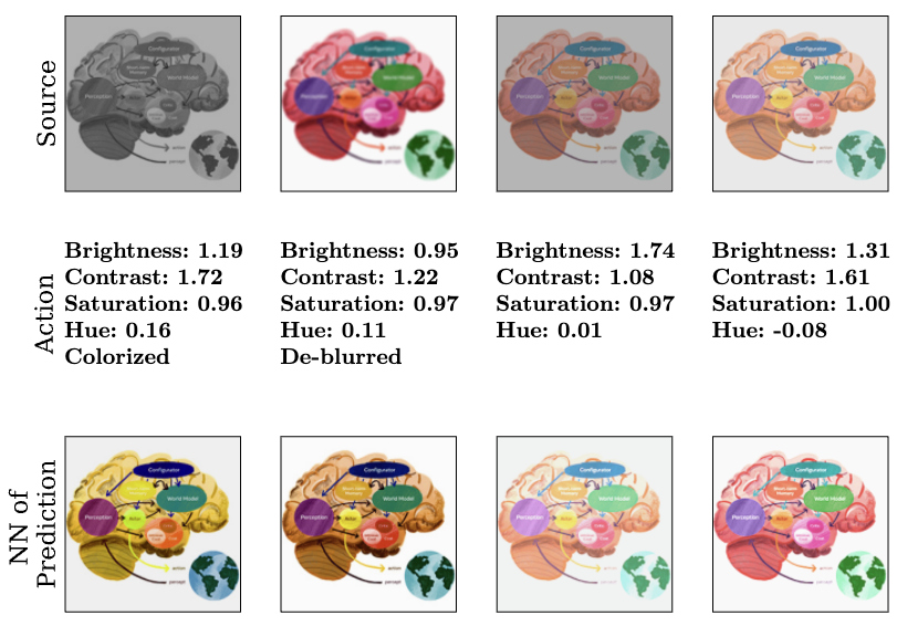
This work introduces Image World Models (IWM). IWM extends I-JEPA by using various image distortions beyond simple masking—such as changes to brightness, contrast, and saturation. These distortions are commonly used in contrastive SSL methods. The action becomes a representation of the distortion applied to the source image to produce the target image. Using the source latent and the action, the IWM predicts the latent representation of the target image.

Since this work focuses solely on images, it lacks a time component. The world that the IWM models exists without a temporal dimension, limiting its application to real-world situations. Additionally, the action space isn’t particularly useful for practical applications. Nevertheless, this approach helps develop richer image representations than those from I-JEPA, which relies exclusively on masking. Distortions are often used to make the image representations invariant to them. However, in this use case, we don’t directly learn invariance but rather the relationships between distorted images. I would classify this method as a great improvement in self supervised representation learning than an advancement in world models.

It is worth noting that many other world model architectures, such as DINO-WM, can be considered Joint Embedding Predicative Architectures (JEPAs).

Conclusion

World models are an important area of research with significant potential. The works described here generally use simple actions, like movement in 2D video games. In the future, we need to model more complex actions at different granularities.

As an example, let’s consider a home robot that does chores. A high-level action would be selecting which chore to start with. This requires considering which task is most important now and how it would affect the household in the near future. Executing the chore requires lower levels of granularity. Say the robot decides to wash dishes, it has to select the order of dishes to wash to optimize storage. And in washing a dish, it has to determine the sequence of mechanical movements to do so effectively and efficiently. We may also need world models that plan for even longer timeframes, like days or months. Our internal world model is powerful, and these kinds of inferences and planning come very easy to us. We underestimate what it would take to replicate this in machines.