L1

https://www.youtube.com/watch?v=2GwBez0D20A&list=PLwRJQ4m4UJjNymuBM9RdmB3Z9N5-0IlY0&index=1&ab_channel=PieterAbbeel

https://www.dropbox.com/scl/fi/rvbpc40ozhstnwhk7h5b7/l1-mdps-exact-methods.pdf?rlkey=5bibe5t8cqmpm9dhth969iiq6&e=1&dl=0

Notation for Markov Decision Processes (MDPs)

Set of states: \(S\)

Start state: \(s_0\) Set of actions: \(A\) Transition function (\(p(s' \vert s, a)\)): Given a state action pair, return the next state. This can be stochastic. Reward function (\(r(s, a, s')\)): Given a state action pair and the resulting next state, return the reward gained. Discount factor (\(\gamma\)): factor to make future rewards valued less than immediate rewards. Horizon (\(H\)): number of actions to take

Objective

Learn a policy \(\pi\) that maps states to actions to maximize the sum of discounted rewards:

\[\max_{\pi} \mathbb{E}_\pi[\sum_{t=0}^{H} \gamma^t R(S_t, A_t, S_{t+1})]\]

Policy can be a deterministic mapping of states to actions \(\pi(s)\). Or we can define a stochastic policy that gives a probability distribution over all actions \(\pi(a\vert s)\).

Value Iteration

Optimal Value Function:

\[V^*(s) = \underset{\pi}{\max} \mathbb{E}\left[∑_{t=0}^{H} γ^t R(s_t, a_t, s_{t+1}) \vert π, s_0 = s\right]\]

Given the optimal infinite horizon policy, what is the expected discounted sum of rewards from a state.

Value iteration is an algorithm to determine the optimal values which can be used to get the optimal policy. The values of all states are initialized to 0. We then loop over all states several times and update the values based on the following rule:

\[V_k^*(s) = \max_{a} \sum_{s'} P(s'|s, a) \left( R(s, a, s') + \gamma V_{k-1}^*(s') \right)\]

The values are initialized to 0, and are updated by looking ahead to the values of the next states. This can be proven to converge to the optimal infinite horizon policy.

Q-Value Iteration

\(Q^*(s,a)\): expected utility from taking an action and a state and acting optimally after

\[Q^{*}(s, a) = \sum_{s'} P(s'\vert s, a)(R(s, a, s') + \gamma \max_{a'} Q^{*}(s', a'))\]

Q-value iteration works similarly to value iteration but with the following update rule:

\[Q_{k+1}(s, a) \leftarrow \sum_{s'} P(s'|s, a) \left( R(s, a, s') + \gamma \max_{a'} Q_k(s', a') \right)\]

Policy Iteration

1. Policy evaluation: run value iteration while fixing the policy
   1. \[V_{i+1}^{\pi_{k}}(s) \leftarrow \sum_{s'} P(s'\vert s, \pi_k(s)) [R(s, \pi_k(s), s') + \gamma V_i^{\pi_k}(s')]\]
2. Policy improvement: redefine policy as taking the best action with one step look ahead
   1. \[\pi_{k+1}(s) \leftarrow \arg \max_a \sum_{s'} P(s'\vert s, a) [R(s, a, s') + \gamma V^{\pi_k}(s')]\]

The key difference between this and value iteration is that we get the action from the policy rather than looping through all possible actions to find the action with the maximum rewards. Policy iteration is generally more efficient.

Maximum Entropy Formulation

The policy incorporates higher entropy to encourage exploration. This approach replaces the standard max operation with a temperature-scaled softmax. Instead of always selecting the optimal action, the agent occasionally chooses suboptimal actions to better explore the state-action space.

L2

https://www.youtube.com/watch?v=Psrhxy88zww&list=PLwRJQ4m4UJjNymuBM9RdmB3Z9N5-0IlY0&index=6

Value iteration and policy iteration are exact methods. They are two limitations:

• Requires access to the dynamics model, this is the exact probabilities of the next state given a current state and action
• Requires iterating over all states and actions. This search space can become prohibitively large.

To remove the dependency on the dynamics model, we can rewrite Q-value iteration as an expectation and same states to estimate this expectation.

\[Q_{k+1} \leftarrow \mathbb{E}_{s' \sim P(s'|s,a)} \left[ R(s, a, s') + \gamma \max_{a'} Q_k(s', a') \right]\]

This no longer depends on the transition probabilities \(P(s'\vert s, a)\). To implement this, we can estimate from samples. Given a state \(s\) and action \(a\) we can sample the next state from the environment \(s'\). We can calculate a target Q-value given this state.

\[\text{target}(s') = R(s, a, s') + \gamma \max_{a'} Q_k(s', a')\]

This is a one sample estimate. We want to estimate using many samples to actually learn from the environment. We can continuously sample states and use an exponential moving average to update the Q-values.

\[Q_{k+1}(s,a) \leftarrow (1 - \alpha)Q_{k}(s,a) + \alpha \left[ \text{target}(s') \right]\]

Over time we want the Q-function that outputs values that are close to the targets. The Q function is implemented as a table storing values for every state action pair. Hence, this is a tabular method.

This approximation solves the first problem of the exact methods since we use sampling rather than exact state transition probabilities. However, we want to also implement a non-tabular version of this so we can scale to larger state and action spaces. Many problems have far too many states to store in a table. Another limitation of tabular methods is that there is no transfer learning between similar states. Some states may be visited more than others and have better converged Q-values.

Actions are chosen greedily based on q-values with \(\epsilon\) probability of choosing a random action for exploration. This is called \(\epsilon\)-Greedy. Q-learning also requires an effective learning rate schedule to reach convergence.

Approximate Q-Learning replaces the table used in tabular Q-Learning a parameterized Q function: \(Q_{\theta}(s,a)\). This function can be represented by any kind of ML model, including neural networks.

This function can be learned by sampling states, and then applying a gradient update to the parameters. The loss is designed so that the output of the Q function matches the target. The target is calculated in the same way as in tabular Q-Learning. The Q function is parameterized by \(\theta_k\) rather than a table.

\[\text{target}(s') = R(s, a, s') + \gamma \max_{a'} Q_{θ_k}(s', a')\] \[θ_{k+1} \leftarrow θ_k - α ∇_θ \left[ \frac{1}{2}(Q_θ(s, a) - \text{target}(s'))^2 \right]\]

The update is a simple least squares regression loss with learning rate \(\alpha\).

DQN

Arxiv paper, Nature paper

Deep Q Learning (DQN) uses a deep neural network to implement the Q function. To align with deep learning principles, it employs large-scale training data and mini-batch optimization.

The algorithm maintains a replay memory \(D\) with capacity \(N\). This is a dataset of past experiences. This allows continuous training on previous experiences to prevent forgetting and ensure that we are training over a large state action space. The memory stores transitions as tuples of (state, action, next state, reward), containing all parameters needed to calculate Q values and targets.

In Atari environments, the environment provides 2D image observations. After taking action \(a_t\), the agent receives a reward \(r_t\) and an image representing the next state \(x_{t+1}\). The next state \(s_{t+1}\) is represented as the tuple \((s_t,a_t,x_{t+1})\). A function \(\phi\) processes this into a state representation \(\phi_{t+1}=\phi(s_{t+1})\). This process reduces the dimensionality of the input data into a compact vector representation. In the Atari implementation, \(\phi\) takes the \(m\) most recent frames and downsamples them from (210x160x128) to (84x84x4) using simple heuristics.

During learning, the agent selects actions using an \(\epsilon\)-Greedy strategy based on the current Q-function. At each step \(t\), the environment generates the next state \(s_{t+1}\) from the current state \(s_t\) and action \(a_t\). After applying \(\phi\), the tuple \((\phi_t, a_t, r_t, \phi_{t+1})\) is stored in \(D\). The algorithm then samples a mini-batch of transitions from \(D\), calculates target values for each transition as labels, and updates the \(Q\) function using these targets. For terminal states, the target value equals the reward. The \(Q\) model updates through gradient descent on the cumulative loss.

The algorithm maintains two Q functions: \(Q\) and \(\hat{Q}\), initialized with identical parameters. While \(\hat{Q}\) calculates targets, \(Q\) receives gradient updates. Every \(C\) steps, \(\hat{Q}\) is synchronized with \(Q\). This lagging version of \(Q\) stabilizes training by reducing target distribution shifts.

The Atari implementation included several optimizations: RMSProp optimizer instead of vanilla SGD, Huber loss in place of squared loss, and \(\epsilon\) annealing to gradually reduce exploration.

Double DQN

When selecting the optimal action in target values, there is a bias toward actions with higher Q-values. Some actions become overestimated while others become underestimated. The argmax in the target function selects only the overestimated actions, creating a bias. This bias can compound as overestimated actions become even more overestimated.

To correct this, we use different parameters for selecting and evaluating the best action. Recall we have two Q functions \(Q\) and \(\hat{Q}\) parametrized by \(\theta\) and \(\theta^-\) respectively. \(\theta\) selects the best action in target, while \(\theta^-\) gets the actual Q-value. The target is reformulated with the following equivalence.

\[\max_{a'} Q(s', a') = Q(s', \argmax_{a'}Q(s', a'))\]

On the right hand side, we use different parameters for the inner and outer instances of the Q function:

\[L_i(\theta_i) = \mathbb{E}_{s, a, s', r} D \left( \left( r + \gamma Q(s', \arg \max_{a'} Q(s', a'; \theta);\theta_i^-) - Q(s, a; \theta_i) \right) \right)^2\]

The outer Q function with \(\theta^-\) doesn’t need to output the highest Q-value for the state since the max is determined separately. This breaks the correlation and reduces the bias of the loss.

Prioritized Experience Replay

In the standard DQN algorithm, all transitions are sampled with equal probability. This modification changes this to sample based on absolute Bellman error:

\[\left| r + \gamma \max_{a'} Q(s', a'; \theta^-) - Q(s, a; \theta) \right|\]

This means that transitions with a larger target discrepancy are sampled more often. These are the more difficult transitions that need more updates to learn. This leads to faster training.

Tutorials

https://pytorch.org/tutorials/intermediate/reinforcement_q_learning.html

L3

https://www.youtube.com/watch?v=AKbX1Zvo7r8&list=PLwRJQ4m4UJjNymuBM9RdmB3Z9N5-0IlY0&index=3

Deep Q-Learning is off policy and is data efficient. On-policy methods can be superior if it is inexpensive to generate more experiences.

Stochastic policy (\(\pi_{\theta}(u\vert s)\)): for each state a model parameterized by \(\theta\) outputs a probability distribution of possible actions \(u\) at state \(s\). The parameters are optimized to maximize expected rewards. Stochastic policies are easier to optimize and also enable better exploration.

Sometimes policies are easier to define than Q or value functions. Q-learning also requires looping over all actions which may be infeasible with large action spaces.

Likelihood Ratio Policy Gradient

\(\tau\) denotes a state action sequence or trajectory: \(s_o,u_0,…,s_H,u_H\)

\(R(\tau)\) is the reward from the sequence \(\sum_{t=0}^HR(s_t,u_t)\)

\(U\) represents the expected rewards under a policy parameterized by \(\theta\). It is the sum of rewards of trajectories weighted by the probability of the trajectory under the policy. We want to use this to optimize \(\theta\). We want policies that have higher probabilities for trajectories with high reward.

\[U(\theta) = \mathbb{E}\left[\sum_{t=0}^{H} R(s_t, u_t); \pi_{\theta}\right] = \sum_{\tau} P(\tau; \theta) R(\tau)\]

We take the gradient of \(U\) with respect to \(\theta\). We want to reformulate the gradient as an expectation so that we can sample values to estimate it. In step 3 the numerator and denominator are multiplied by \(P(\tau; \theta)\) to turn the gradient into a weighted sum. We get the logarithm by applying the chain rule in reverse \(\frac{1}{f(x)} \cdot f'(x) = \frac{d}{dx} \ln(f(x))\).

\[\begin{align*}\nabla_{\theta} U(\theta) &= \nabla_{\theta} \sum_{\tau} P(\tau; \theta) R(\tau) \\&= \sum_{\tau} \nabla_{\theta} P(\tau; \theta) R(\tau) \\&= \sum_{\tau} \frac{P(\tau; \theta)}{P(\tau; \theta)} \nabla_{\theta} P(\tau; \theta) R(\tau) \\&= \sum_{\tau} P(\tau; \theta) \frac{\nabla_{\theta} P(\tau; \theta)}{P(\tau; \theta)} R(\tau) \\&= \sum_{\tau} P(\tau; \theta) \nabla_{\theta} \log P(\tau; \theta) R(\tau) \\\end{align*}\]

We want to estimate the gradient using samples. We can have a minibatch of \(m\) samples and use the following formula to estimate the gradient. We also now have log probabilities which are numerically stable. From the derivation we can rewrite the gradient as a estimated expectation with \(m\) samples:

\[\begin{align*} \nabla_{\theta} U(\theta) &\approx \hat{g} = \frac{1}{m} \sum_{i=1}^{m} \nabla_{\theta} \log P(\tau^{(i)}; \theta) R(\tau^{(i)}) \end{align*}\]

This does not require the reward function to be known or differentiable. The sample space can also be discrete. We only require the parameters to be differentiable.

Temporal Decomposition

So far, we are shifting the probabilities of entire trajectories. However, we may want be more localized and shift parts of the trajectories.

To understand how the policy gets updated, we can decompose the trajectory probabilities.

\[\begin{align*}\nabla_{\theta} \log P(\tau^{(i)}; \theta) &= \nabla_{\theta} \log \left[ \prod_{t=0}^{H} \underbrace{P(s_{t+1}^{(i)}|s_{t}^{(i)}, u_{t}^{(i)})}_{\text{dynamics model}} \cdot \underbrace{\pi_{\theta}(u_{t}^{(i)}|s_{t}^{(i)})}_{\text{policy}} \right] \\&= \nabla_{\theta} \sum_{t=0}^{H} \left[ \log P(s_{t+1}^{(i)}|s_{t}^{(i)}, u_{t}^{(i)}) + \log \pi_{\theta}(u_{t}^{(i)}|s_{t}^{(i)}) \right] \\&= \nabla_{\theta} \sum_{t=0}^{H} \log \pi_{\theta}(u_{t}^{(i)}|s_{t}^{(i)}) \\&= \sum_{t=0}^{H} \nabla_{\theta} \log \pi_{\theta}(u_{t}^{(i)}|s_{t}^{(i)})\end{align*}\]

Since the dynamics model term doesn’t depend on \(\theta\), we can drop it from the equation. This reformulation shows how policy gradients work: they learn to increase probabilities for state-action pairs that lead to higher rewards while decreasing probabilities for pairs that lead to lower rewards. Through sampling multiple trajectories, this approach gradually learns effective policies.

Baseline Subtraction

In the default formulation, trajectories with positive rewards always have their probabilities increased. Over time, trajectories with higher rewards dominate those with lower rewards. Only trajectories with negative rewards have their probabilities decreased. However, we want to decrease the probabilities of trajectories that perform below average. This is important because in some environments, all trajectories might have only positive rewards or only negative rewards. Baseline subtraction addresses this by centering the trajectory rewards around 0, which enables more effective learning by reducing the variance of the gradients.

We simply subtract a baseline \(b\) from all trajectory rewards: \(R(\tau^{(i)})-b\). This baseline value cannot depend on the parameters \(\theta\) as to not affect the gradients.

Temporal Structure on Rewards

We can also decompose the rewards based on the time. We also split the past rewards and expected future rewards.

\[\begin{align*}\hat{g} &= \frac{1}{m} \sum_{i=1}^{m} \nabla_{\theta} \log P(\tau^{(i)}; \theta) \left( R(\tau^{(i)}) - b \right) \\&= \frac{1}{m} \sum_{i=1}^{m} \left( \sum_{t=0}^{H-1} \nabla_{\theta} \log \pi_{\theta}(u_{t}^{(i)}|s_{t}^{(i)}) \right) \left( \sum_{t=0}^{H-1} R(s_{t}^{(i)}, u_{t}^{(i)}) - b \right) \\&= \frac{1}{m} \sum_{i=1}^{m} \left( \sum_{t=0}^{H-1} \nabla_{\theta} \log \pi_{\theta}(u_{t}^{(i)}|s_{t}^{(i)}) \right) \left[ \left( \sum_{k=0}^{t-1} R(s_{k}^{(i)}, u_{k}^{(i)}) \right) + \left( \sum_{k=t}^{H-1} R(s_{k}^{(i)}, u_{k}^{(i)}) - b \right) \right]\end{align*}\]

The first reward term can be removed since past rewards don’t depend on the current action.

\[\frac{1}{m} \sum_{i=1}^{m} \sum_{t=0}^{H-1} \nabla_{\theta} \log \pi_{\theta}(u_{t}^{(i)}|s_{t}^{(i)}) \left( \sum_{k=t}^{H-1} R(s_{k}^{(i)}, u_{k}^{(i)}) - b(s_{t}^{(i)}) \right)\]

The baseline values can depend on the current state.

Baseline Choices

• Constant baseline: average rewards of all trajectories
  • \[b = \mathbb{E}[R(\tau)] \approx \frac{1}{m} \sum_{i=1}^{m} R(\tau^{(i)})\]
• Optimal Constant baseline: Weight rewards of trajectories by the squared gradient probabilities of the trajectory
  • Shown mathematically to reduce variance but not commonly used
  • \[b = \frac{\sum_{i=1}^{m} \left( \nabla_{\theta} \log P(\tau^{(i)}; \theta) \right)^2 R(\tau^{(i)})}{\sum_{i=1}^{m} \left( \nabla_{\theta} \log P(\tau^{(i)}; \theta) \right)^2}\]
• Time-dependent baseline: Average rewards after the current timestep.
  • This accounts for changes in the expected rewards in different points in the trajectories. This is the same as the constant baseline, but filtered on the timestep.
  • \[b_t = \frac{1}{m} \sum_{i=1}^{m} \sum_{k=t}^{H-1} R(s_{k}^{(i)}, u_{k}^{(i)})\]
• State-dependent expected return baseline:
  • Rewards from the state given the current policy. This computes the value function of the state and uses it as the baseline.
  • The updates are higher if the rewards are higher than that of the current policy. This is intuitive in that updates are scaled based on the difference with the current policy.
  • \[b(s_t) = \mathbb{E}\left[r_t + r_{t+1} + r_{t+2} + ... + r_{H-1} \right] = V^{\pi}(s_t)\]

Value Function Estimation

Monte-Carlo estimation of \(V^{\pi}(s_t)\). We parameterize \(V\) with \(\phi\), which can be a neural network. Given \(m\) trajectories under the current policy, we can train the value function with the true rewards as a label.

\[\phi_{i+1} \leftarrow \arg \min_{\phi} \frac{1}{m} \sum_{i=1}^{m} \sum_{t=0}^{H-1} \left( V_{\phi}^{\pi}(s_{t}^{(i)}) - \left( \sum_{k=t}^{H-1} R(s_{k}^{(i)}, u_{k}^{(i)}) \right) \right)^2\]

An alternative to the regression is bootstrap estimation. This is similar to value iteration but with a fixed policy. We want the difference between values of consecutive states to the reward of the transition \(r\). We also regularize the updates to \(\phi\).

\[\phi_{i+1} \leftarrow \min_{\phi} \sum_{(s, u, s', r)} \left\| r + V_{\phi_i}^{\pi}(s') - V_{ϕ}(s) \right\|_2^2 + \lambda \left\| \phi - \phi_i \right\|_2^2\]

Vanilla Policy Gradient Algorithm

1. Initialize a policy \(\theta\)
2. At each iteration sample \(m\) trajectories from the current policy
3. Compute the rewards \(R_t\) and the advantage estimate \(\hat{A}_t = R_t-b(s_t)\) at each timestep of each trajectory.
4. Update the value function / baseline using either Monte-Carlo estimation or bootstrap estimation.
5. Update the policy at the end of each iteration using the policy gradient \(\hat{g}\).
   1. Sum for each trajectory and timestep: \(\nabla_{\theta} \log \pi(a_t \vert s_t, \theta) \hat{A}_t\)

Advantage Estimation

We want to improve our calculation of the rewards from taking an action: \(\sum_{k=t}^{H-1} R(s_{k}^{(i)}, u_{k}^{(i)})\). This can also be referred to as \(Q^{\pi}(s,u)\).

The simplest way is to just roll out the trajectory and add up the rewards:

\[Q^{\pi}(s,u)=\mathbb{E}[r_0+r_1+r_2+...|s_0 = s, a_0=a]\]

Since this is based on a single trajectory, this has high variance.One way to reduce the variance is by using a discount factor \(\gamma\) for the sum of rewards can reduce the variance of the gradients. This is an inductive bias assuming that actions lose their effect over time.

\[Q^{\pi,\gamma}(s,u)=\mathbb{E}[ r_0+\gamma r_1+\gamma^2r_2+...|s_0 = s, a_0=a]\]

We can also replace the rollout with a value function estimate:

\[Q^{\pi,\gamma}(s,u)=\mathbb{E}[ r_0+\gamma V^{\pi}(s_1)|s_0 = s, a_0=a]\]

We can also interpolate between these two formulas by rolling out \(k\) steps and then using the value function.

\[Q^{\pi,\gamma,k}(s,u)=\mathbb{E}[ r_0+\gamma r_1+...+\gamma^{k-1}r_k+\gamma^k V^{\pi}(s_{k+1})|s_0 = s, a_0=a]\]

This method is called Async Advantage Actor Critic (A3C). This method is asynchronous because there are multiple actors using the policy and asynchronously updating the parameters. Advantage Actor Critic (A2C) is a synchronous version that averages updates across multiple trajectories from different actors. These are called actor-critic methods because they use two models: a policy network acting as the actor and a value function serving as the critic that evaluates the actor’s actions.

Generalized Advantage Estimation (GAE) is an exponentially weighted average (weighted by \(\lambda\)) of this function with different \(k\) values. This calculation can be performed efficiently. We can represent this as \(Q^{\pi,\gamma,k,\lambda}(s,u)\)

We can update the vanilla policy gradient algorithm to support these actor critic methods:

1. Initialize a policy parameterized by \(\theta_0\) and a value function parameterized by \(\phi_0\)
2. At each iteration sample \(m\) trajectories from the current policy
3. Update the value function / baseline at each timestep using the actor critic estimate for the Q value (\(\hat{Q}_i(s, u)\)):
   1. \[\phi_{i+1} \leftarrow \phi_i - \alpha_{\phi} \frac{1}{m} \sum_{k=1}^{m} \sum_{t=0}^{H-1} \nabla_{\phi} \left[ \Vert \hat{Q}_i(s_t^{(k)}, u_t^{(k)}) - V_{\phi}^{\pi}(s_t^{(k)}) \Vert _2^2 + \kappa \Vert \phi - \phi_i \Vert _2^2 \right]\]
4. Update the policy also using the estimate for Q-Value. This is averaged across the \(m\) trajectories.
   1. \[\theta_{i+1} \leftarrow \theta_i + \alpha_{\theta} \frac{1}{m} \sum_{k=1}^m \sum_{t=0}^{H-1} \nabla_{\theta} \log \pi_{\theta_i}(u_t^{(k)} \vert s_t^{(k)}) \left( \hat{Q}_i(s_t^{(k)}, u_t^{(k)}) - V_{\phi_i}^{\pi}(s_t^{(k)}) \right)\]

We are optimizing two neural networks in parallel with separate learning rates \(\alpha_{\phi}\) and \(\alpha_{\theta}\).

More details on Policy Gradient Methods: https://lilianweng.github.io/posts/2018-04-08-policy-gradient/

L4

https://www.youtube.com/watch?v=KjWF8VIMGiY&list=PLwRJQ4m4UJjNymuBM9RdmB3Z9N5-0IlY0&index=4

We can derive policy gradients from importance sampling. Importance sampling allows us to evaluate a new policy \(\theta\) using data collected from an old policy \(\theta_{old}\). To estimate the expected return \(U(\theta)\) of the new policy, we multiply each trajectory’s reward by an importance weight \(\frac{P(\tau\vert \theta)}{P(\tau\vert \theta_{\text{old}})}\). This weight increases the weight of trajectories that are more likely under the new policy and decreases the weight of those that are less likely.

\[U(\theta) = \mathbb{E}_{\tau \sim \theta_{\text{old}}} \left[ \frac{P(\tau|\theta)}{P(\tau|\theta_{\text{old}})} R(\tau) \right]\]

We can then take the gradient to update the policy to increase the rewards.

\[\begin{align*} \nabla_{\theta} U(\theta) &= \mathbb{E}_{\tau \sim \theta_{\text{old}}} \left[ \frac{\nabla_{\theta} P(\tau|\theta)}{P(\tau|\theta_{\text{old}})} R(\tau) \right] \\[10pt] \nabla_{\theta} U(\theta)|_{\theta=\theta_{\text{old}}} &= \mathbb{E}_{\tau \sim \theta_{\text{old}}} \left[ \frac{\nabla_{\theta} P(\tau|\theta)|_{\theta=\theta_{\text{old}}}}{P(\tau|\theta_{\text{old}})} R(\tau) \right] \\[10pt] &= \mathbb{E}_{\tau \sim \theta_{\text{old}}} \left[ \nabla_{\theta} \log P(\tau|\theta)|_{\theta=\theta_{\text{old}}} R(\tau) \right] \end{align*}\]

We can estimate this expectation by sampling trajectories from the old policy to obtain a policy gradient for updating \(\theta\). A key insight is that \(\theta_{old}\) need not be the current policy. When it is the current policy, this reduces to vanilla policy gradients. This flexibility proves valuable when we want to perform multiple gradient updates using a single batch of sampled trajectories.

Step Size

Small step sizes may prevent reaching a good policy, especially under data constraints. Large step sizes can result in being stuck in bad policies.

Simple step-sizing: linear search in the direction of the gradient by trying different values for the step size. This is simple but expensive as it requires many policy evaluations for a single update. It is also limited as a first-order approximation.

Trust Region Policy Optimization (TRPO)

We use the importance sampling ratio to perform multiple updates from a single set of trajectories under an old policy. This is a higher order approximation.

We optimize a surrogate loss using the old policy:

\[\max_{\pi} L(\pi) = \mathbb{E}_{\pi_{\text{old}}} \left[ \frac{\pi(a|s)}{\pi_{\text{old}}(a|s)} A^{\pi_{\text{old}}}(s, a) \right]\]

We also want to constrain the updates. The importance sampling ratio is only accurate when the current policy is near the old policy. When they drift apart, we would want to resample trajectories. We check the following constraint:

\[\mathbb{E}_{\pi_{\text{old}}} \left[ KL(\pi||\pi_{\text{old}}) \right] \leq \epsilon\]

We check this constraint as we are doing the line search and use it to determine when to start a new iteration.

The algorithm as a whole:

1. Sample \(N\) trajectories for \(T\) timesteps
2. Estimate the advantage under the old policy at each step.
3. Compute the policy gradient \(g\)
4. [Optional] Use conjugate gradients to calculate a natural policy gradient \(F^{-1}g\)
   1. \(F\) is the Fisher Information Matrix which represents the curvature of the policy functions. We want to find the solution to \(Fx=g\) which is \(F^{-1}g\).
   2. \(F\) is of size \([d_{\theta},d_{\theta}]\) where \(d_{\theta}\) is the number of parameters in the policy model. This is prohibitively expensive. Conjugate gradients is an iterative method to approximate \(F^{-1}g\) without materializing \(F\).
   3. This method doesn’t directly utilize the constraint. Rather, it uses a second order approximation to optimize the policy while accounting for the curvature. This kind of optimization tends to improve the policy while not increasing the KL divergence as much as the standard policy gradient.
5. Do a line search on the gradient (using the policy or natural policy gradient) direction to update the parameters as much as possible while still meeting the constraint.

The KL constraint can be evaluated as follows:

\[\begin{align*} KL(P(\tau;\theta)||P(\tau;\theta+\delta\theta)) &= \sum_{\tau} P(\tau;\theta) \log \frac{P(\tau;\theta)}{P(\tau;\theta+\delta\theta)} \\ &= \sum_{\tau} P(\tau;\theta) \log \frac{P(s_0) \prod_{t=0}^{H-1} \pi_{\theta}(u_t|s_t)P(s_{t+1}|s_t,u_t)}{P(s_0) \prod_{t=0}^{H-1} \pi_{\theta+\delta\theta}(u_t|s_t)P(s_{t+1}|s_t,u_t)} \\ &= \sum_{\tau} P(\tau;\theta) \log \frac{\prod_{t=0}^{H-1} \pi_{\theta}(u_t|s_t)}{\prod_{t=0}^{H-1} \pi_{\theta+\delta\theta}(u_t|s_t)} \\ &= \mathbb{E}_{\tau \sim \theta} \log \frac{\prod_{t=0}^{H-1} \pi_{\theta}(u_t|s_t)}{\prod_{t=0}^{H-1} \pi_{\theta+\delta\theta}(u_t|s_t)} \\ &\approx \frac{1}{M} \sum_{(s,u) \text{ in roll-outs under } \theta} \log \frac{\pi_{\theta}(u|s)}{\pi_{\theta+\delta\theta}(u|s)}\end{align*}\]

We unroll the probabilities of the trajectories using the dynamics model \(P(s_{t+1}\vert s_t,u_t)\). However, this term cancels out since it doesn’t depend on the policy parameters \(\theta\). We then get that an expectation on the old policy of the log ratios between the predictions of the two policies. We can approximate this expectation with M samples from the old policy. \(\theta\) corresponds to \(\pi_{old}\), while \(\theta+\delta\theta\) corresponds to the new policy being evaluated.

OpenAI TRPO Documentation

Proximal Policy Optimization (PPO)

PPO is currently one of the most popular RL algorithms. It is commonly used for RLHF. It is an improvement upon TRPO. Rather than conjugate gradients, we want to use first-order optimizers like Adam and RMSProp. This makes PPO more effective with deep learning model architectures.

PPO V1 (Dual Descent TRPO)

\[\max_\theta \hat{\mathbb{E}}_t \left[ \frac{\pi_\theta(a_t|s_t)}{\pi_{\theta_\text{old}}(a_t|s_t)} \hat{A}_t \right] - \beta \left( \hat{\mathbb{E}}_t \left[ \text{KL}[\pi_{\theta_\text{old}}(\cdot|s_t), \pi_\theta(\cdot|s_t)] \right] - \delta \right)\]

At each iteration of the policy gradient algorithm, we train with SGD for a certain number of epochs.

From TRPO, we move the constraint into the loss. However, this requires the right choice of \(\beta\). This parameter is the Lagrange multiplier or dual variable. After \(\theta\) is updated, we use the KL value to determine whether to increase or decrease \(\beta\). There is a formal process for these updates.

This algorithm shows how first order optimizers can be used to train TRPO while meeting the KL constraint.

PPO V2 (Clipped Surrogate Loss)

We define the probability ratio \(r_t\) as a function of \(\theta\):

\[\quad r_t(\theta) = \frac{\pi_\theta(a_t|s_t)}{\pi_{\theta_\text{old}}(a_t|s_t)}\]

This leads to the following objective:

\[L^{\text{CLIP}}(\theta) = \hat{\mathbb{E}}_t \left[ \min(r_t(\theta)\hat{A}_t , \text{clip}(r_t(\theta), 1 - \epsilon, 1 + \epsilon)\hat{A}_t ) \right ]\]

Inside the expectation, we compare two terms: the unclipped ratio \(r_t(\theta)\) (as in PPO V1) and the clipped ratio, both multiplied by the advantage \(\hat{A}_t\).

When the ratio falls outside the clipping bounds, the importance sampling ratio becomes unreliable, so we reduce the update to \(\theta\). We say that for a given state action pair, when the ratio of the new policy exceeds the \(\epsilon\) bounds, there is nothing further to learn. When the loss is clipped there is no derivative with respect to \(\theta\) so there is no update on these timesteps. These timesteps are further trained in subsequent iterations with updated \(\pi_{old}\). The update only occurs when the ratio stays within bounds, naturally enforcing the KL constraint. By taking the minimum between the clipped and unclipped ratios, we ensure conservative updates.

We need to consider the signs of the ratios and advantages. When both are positive, we increase the probability of good actions, and when both are negative, we decrease the probability of bad actions. The clipping mechanism limits both types of updates. However, edge cases occur when the signs don’t match. In these situations, the min operation might select the term with the larger absolute value (for example, when \(r_t<1-\epsilon\) and \(\hat{A}_t > 0\)). The presented clipping formula is somewhat simplified and inaccurate. In practice, the clipping behavior depends on the advantage’s sign.

source

This mechanism ensures proper clipping based on both the ratio and advantage’s absolute values.

This approach simplifies the optimization objective by eliminating the need to update \(\beta\). Instead, we only need to tune the hyperparameter \(\epsilon\). The purpose behind the KL constraint and clipping is to only update the policy in a trusted region around the old policy where the data is collected.

L5

https://www.youtube.com/watch?v=pg-lKy7JIRk&list=PLwRJQ4m4UJjNymuBM9RdmB3Z9N5-0IlY0&index=5

Off policy methods are more sample efficient. We can learn more from fewer samples, but with more computation used for learning.

Deep Deterministic Policy Gradient (DDPG)

DDPG can be viewed as a policy gradient version of DQN. Like with policy gradients, we sample \(m\) rollouts in an iteration. We add noise to these sampled rollouts for exploration.

Q function update

We calculate target Q values with a one step rollout.

\[\hat{Q}(s_t, u_t) = r_t + \gamma Q_\phi(s_{t+1}, u_{t+1})\]

Optionally, we can use lagged Polyak-averaged parameters \(\phi'\), \(\theta'\) to compute the target Q values. This is similar to what we do in DQN for training stability.

\[\hat{Q}_t = r_t + \gamma Q_{\phi'}(s_{t+1}, \pi_{\theta'}(s_{t+1}))\]

With these target values, we update the parameters of the Q function with a regression loss.

\[g \propto \nabla_\phi \sum_t (Q_\phi(s_t, u_t) - \hat{Q}(s_t, u_t))^2\]

Policy update

Using the updated Q function, we update the policy.

\[g \propto \sum_t \nabla_\theta Q_\phi(s_t, \pi_\theta(s_t, v_t))\]

This is similar to Q value iteration, but while increasing the probability of actions with higher Q values. We can also use a replay buffer to train on trajectories for more iterations. Unlike in DQN, we have separate models for Q and the policy, which makes this an actor critic method. Since we have a separate policy model, this works with continuous actions and we don’t have to iterate over a discrete action space.

Soft Actor Critic (SAC)

This method is the maximum entropy version of DDPG. We maximize the entropy of the policy in the objective.

In the target Q value calculation, we subtract the log probability of the action under the policy. This increases the entropy of Q values with respect to the probabilities of the actions. High probability actions will be closer to lower probability ones.

\[\hat{Q_i}(s_t, u_t) = r_t + \gamma( Q_{\phi_i}(s_{t+1}, u_{t+1})-\alpha\log\pi_{\theta}(u_t|s_t))\]

SAC also uses two Q functions / critics \(\phi_1\), \(\phi_2\) to improve stability. We take the minimum Q value:

\[\hat{Q}(s_t, u_t)=\min_{i=1,2}\hat{Q_i}(s_t, u_t)\]

The policy is updated using the updated Q functions. We also subtract the log probability and take the minimum:

\[g \propto \sum_t \nabla_\theta \min_{i=1,2}Q_{\phi_i}(s_t, a_\theta(s_t, v_t)) -\alpha\log\pi_{\theta}(a_{\theta}(s_t)|s_t))\]

This gradient optimizes the KL divergence of the new policy’s actions with respect to the normalized old policy’s Q values:

\[\mathrm{D}_{\mathrm{KL}} \left( \pi_{\theta}(\cdot|s) \left\| \frac{1}{Z} \exp Q^{\pi_{\theta_{old}}}(s, \cdot) \right. \right)\]

We sample actions from the policy to perform this update. Like DDPG, we can use a replay buffer and sample transitions.

OpenAI Documentation

L6

https://www.youtube.com/watch?v=2o1yrkbpcUk&list=PLwRJQ4m4UJjNymuBM9RdmB3Z9N5-0IlY0&index=6

Algorithm

At each iteration:

1. Collect data with the current policy
2. Learn a dynamics model from past data
3. Improve the policy using the updated dynamics model

We can use the model to simulate experiences to learn the policy from. Model-based RL has better sample efficiency but can be unstable to train. There is also less convergence in the community to specific methods. The model can also be reused for different tasks in an environment.

The model can be a neural network representation of the transitions given a state and an action: \(P(s'\vert s, a)\), \(R(s, a, s')\).

These algorithms are best understood through code rather than math.

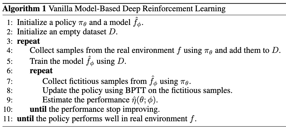
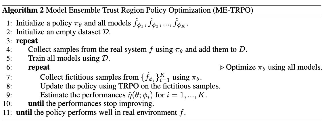
Model Ensemble Trust Region Policy Optimization

This addresses the problem of the policy overfitting in regions where the model is undertrained. We want to avoid overfitting to the model’s bias.

An ensemble of models can be used to determine whether the models are confident. Areas where the models in the ensemble disagree represents regions that need more model training. By training with an ensemble of models, the updates in the areas of disagreement will cancel out.

We first sample trajectories from the real environment using the policy and train the models. We then have a loop where we sample trajectories using each of the models in the ensemble. This is used to train the policy using TRPO. We keep iterating this sampling and training process until the performance of the policy with respect to each model’s simulated trajectories stops improving. We iterate on this to improve the policy with interactions with the real environment.

Model-based via Meta-Policy Optimization MB-MPO

The goal is to learn an adaptive policy that can adapt to any learned model in the ensemble.

We learn an “adapted policy” \(\theta'_k\) for each model in the ensemble. We sample trajectories from the real environment using each adapted policy, and a train a model \(\phi_k\). We then sample simulated trajectories from the learned model and update the adapted model. The unadapted policy \(\theta\) is updated with the averaged gradient across these adapted policies with their respective simulated trajectories.

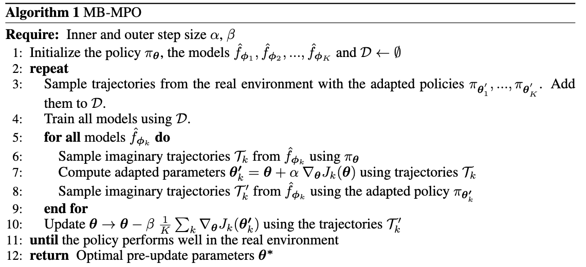
The adapted policies \(\theta'_k\) are set to be one gradient step from the unadapted policy \(\theta\). This objective learns an unadapted policy that can easily adapt to different models. With an adaptation step size \(\alpha\) of 0, this is similar to ME-TRPO.