Lecture Notes: https://diffusion.csail.mit.edu/docs/lecture-notes.pdf

Lab One

Lab Two

Lab Three

Generative Modeling

The quality of a generation can be interpreted as the probability than the generated object came from a target distribution. For example, if you are generating images of dogs we want to measure the probability it came from the distribution of dog images.

The probability distribution can be represented as a mapping from vectors to non negative numbers.

\[p_{\mathrm{data}}: \mathbb{R}^d \rightarrow \mathbb{R}_{\geq0}\]

We can’t explicitly define \(p_{\mathrm{data}}\) but we can access samples from it (dataset): \(z_1, z_2, \ldots, z_n \sim p_{\mathrm{data}}\).

Unconditional generation (sampling from the data distribution):

\[z \sim p_{\mathrm{data}}\]

Conditional generation (conditioning the sampling with \(y\), which can be a prompt):

\[z \sim p_{\mathrm{data}}(\cdot|y)\]

The data distribution is randomly initialized:

\[p_{\text{init}} = \mathcal{N}(0, I_d)\]

The generative model transforms this into the data distribution.

Flow Models

Trajectory

This is a function of time mapping to a vector. Time is constrained to be between 0 and 1. We can call each step in the trajectory \(X_t\) as a state (similar to RL terminology).

\[X:[0,1] \rightarrow \mathbb{R}^d, t\mapsto X_t\]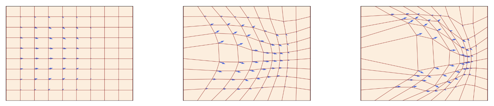

Example of a 2D flow from the lecture notes. The flow here is a grid of trajectories shown at 3 time steps. The flow warps the space of the grid. Red is flow, blue is vector field. the vector field changes over time. Individual points in the grid over time represent trajectories.

Ordinary Differential Equation (ODE)

\[\frac{d}{dt}X_t = u_t(X_t)\]

Initial condition:

\[X_0 = x_0\]

Vector Field

This maps time and location \(x\) to a vector.

\[u:\mathbb{R} \times [0,1] \rightarrow \mathbb{R}^d, (x,t) \mapsto u_t(x)\]

Flow

Collection of trajectories that follow an ODE with different initial conditions.

\[\psi:\mathbb{R}\times[0,1]\rightarrow\mathbb{R}^d,(x,t)\mapsto\psi_t(x_0)\\ \psi_0(x_0)=x_0\\ \frac{d}{dt}\psi_t(x_0) = u_t(\psi_t(x_0))\]

A vector field defines an ODE. A trajectory is a solution. A flow is a collection of solutions.

Picard-Lindelöf theorem: If the vector field is continuously differentiable with bounded derivatives then a solution exists. This is true when the vector field is Lipschitz. In ML, the derivatives of the models are never unbounded so we always get solutions.

ODE Solutions

Closed Form

Some ODEs are solvable by hand like Linear ODEs. Otherwise we can use simulation.

Euler Method

After initializing \(X_0 = x_0\), we can update \(X\) as follows:

\[X_{t+h} = X_t+hu_t(X_t)\quad (t=0,h,2h,3h,…1-h)\]

\(h\) is the step size parameter. We take steps in the direction of the vector field.

Heun’s Method

We use Euler’s method to guess the next state. Then we update \(X\) with the average of the current state and the guess for the new state.

\[X'_{t+h} = X_t + h u_t(X_t) \quad \\X_{t+h} = X_t + \frac{h}{2} (u_t(X_t) + u_{t+h}(X'_{t+h})) \quad\]

Flow Models

We use an ODE to map the initial distribution to the data distribution. The vector field is parameterized by the neural network: \(u_t^{\theta}:\mathbb{R}^d\times[0,1]\to\mathbb{R}^d\)

The neural network model is the vector field. The flow is a result of sampling trajectories.

The goal is to have the have the last state \(X_1\) match the data distribution.

Random initialization: \(X_o \sim p_{\mathrm{init}}\)

ODE: \(\frac{d}{dt} X_t = u_t^{\theta}(X_t)\)

Goal: \(X_1 \sim p_{\mathrm{data}}\)

Diffusion Models

\(X_t\) is a random variable

\[X:[0,1] \rightarrow \mathbb{R}^d, t\mapsto X_t\]

The trajectories are stochastic. We can sample multiple different trajectories.

Vector field: \(u:\mathbb{R} \times [0,1] \rightarrow \mathbb{R}^d, (x,t) \mapsto u_t(x)\)

Diffusion Coefficient: \(\sigma: [0,1] \to \mathbb{R}, t \mapsto \sigma_t\)

The diffusion coefficient injects stochasticity. When it is zero it is deterministic.

Stochastic Differential Equation (SDE)

\[dX_t = u_t(X_t)dt+\sigma_tdW_t\]

Initial condition:

\[X_0=x_0\]

The SDE is the same as the ODE but with a stochastic term. \(\sigma_t\) is the scalar diffusion coefficient.

\(W\) is Brownian motion.

Brownian Motion

Continuous random walk

Stochastic process: \(W=(W_t)_{t\geq0}\)

1. \[W_0 = 0\]
2. Gaussian increments: \(W_t - W_s \sim \mathcal{N}(0,(t-d)I_d)^{(0\leq s \lt t)}\)
3. Independent increments: \(W_{t_1} - W_{t_0}, …, W_{t_n} - W_{t_{n-1}}\) are independent (\(0\geq t_{n-1} \gt t_{n}\))

Brownian motion is a Gaussian process. It is not differentiable because it is stochastic. Even with infinitesimally small increments the increments are stochastic so it is impossible to define a derivative.

State Updates

ODE

If a trajectory has the ODE \(dX_t = u_t(X_t)dt\), we can define the next state using the vector field and an error term \(R_t\).

\[X_{t+h}=X_t+hu_t(X_t)+hR_t(h) \quad \lim_{h\to0}R_t(h) = 0\]

We can rearrange terms to get an approximation of the derivative with \(h\) as the step size.

\[\frac{X_{t+h}-X_t}{h} = u_t(X_t)+R_t(h)\]

In the limit of the step size going to zero, the error term becomes 0 and the vector field defines the derivative.

SDE

We can make this stochastic with the SDE \(dX_t = u_t(X_t)dt +\sigma_tdW_t\).

\[X_{t+h} = X_t+hu_t(X_t)+\sigma_t(W_ {t+h} - W_t) + hR_t(h) \quad \lim_{h\to0}\sqrt{\mathbb{E}[||R_t(h)||^2]}= 0\]

The standard deviation of the error goes to 0.

SDEs also have unique solutions for all vector fields with bounded derivatives and if it is Lipschitz. Additionally the diffusion coefficient has to be continuous.

Sampling from SDE

Euler-Maruyama method

In diffusion models, the initial state is randomly sampled.

For each step:

1. Sample \(\epsilon \sim \mathcal{N}(0,I_d)\)
2. Update the state: \(X_{t+h} = X_t+hu_t^{\theta}(X_t)+\sigma_t\sqrt{h}\epsilon\)
   1. \(\sqrt{h}\) is needed so that the variance scales linearly with \(h\)

Ohrnstein-Uhlenbeck Process

\[dX_t = -\theta X_tdt + \sigma dW_t\]

Solutions to this SDE converge to a Gaussian distribution.

Diffusion Model

We have the same goal as flow models.

Random initialization: \(X_o \sim p_{\mathrm{init}}\)

SDE: \(dX_t = u_t^{\theta}(X_t)dt+\sigma_tdW_t\)

Goal: \(X_1 \sim p_{\mathrm{data}}\)

Summary

Flow Model

Initialize: \(X_0 \sim p_{\text{init}}\)

ODE: \(dX_t = u_t^{\theta}(X_t)dt\)

Diffusion Model

Initialize: \(X_0 \sim p_{\text{init}}\)

SDE: \(dX_t = u_t^{\theta}(X_t)\text{d}t + \sigma_t dW_t\)

Sampling

Simulate from t=0 to t=1 and return \(X_1\).

The only difference is the stochastic component in the updates.

Training Target

We want to construct a target to train the vector field.

\[L(\theta) = \left\| u_t^{\theta}(x) - u_t^{\text{target}}(x) \right\|^2\]

Conditional: per single data points

Marginal: across all data points

Conditional Probability Path

Dirac distribution: distribution always has the same value. \(z\in \mathbb{R}^d, \delta_z, x\sim \delta_z \rightarrow X=z\)

Conditional Probability path: \(p_t(\cdot\vert z)\)

1. \(p_t(\cdot\vert z)\) is a probability distribution over \(\mathbb{R}^d\)
2. Over time the distribution collapses onto a single point. \(p_0(\cdot\vert z) = p_{\text{init}}(\cdot)\), \(p_1(\cdot\vert z) = \delta_z\)

Example: Gaussian probability paths

\[p_t(\cdot\vert z)=\mathcal{N}(\alpha_tz, \beta_t^2I_d)\]

Noise schedulers: \(\alpha_t, \beta_t \quad\text{s.t.}\quad \alpha_0 = 0, \alpha_1 = 1, \beta_0 = 1, \beta_1 = 0\), The variance goes to 0 as the mean goes to the datapoint.

example values: \(\alpha_t = t, \beta_t = 1-t\)

Marginal Probability Path

\[z\sim p_{\text{data}}, x \sim p_t(\cdot\vert z) \rightarrow x\sim p_t\]

We marginalize over \(z\).

1. \[p_t(x) = \int p_t(x\vert z)p_{\text{data}}(z)dz\]
2. \(p_0 = p_{\text{init}}\), \(p_1 = p_{\text{data}}\)

Conditional Vector Field

Definition:

\[u_t^{\text{target}}(x|z), \quad 0\leq t \leq 1, \quad x,z \in \mathbb{R}^d\]

that satisfies

\[X_0 \sim p_{\text{init}}, \quad \frac{d}{dt}X_t = u_t^{\text{target}}(x|z) \rightarrow X_t\sim p_t(\cdot|z) ,\quad 0 \leq t \leq 1\]

Conditional Gaussian Vector Field

\[u_t^{\text{target}}(x \mid z) = \left( \dot{\alpha}_t - \frac{\dot{\beta}_t}{\beta_t} \alpha_t \right) z + \frac{\dot{\beta}_t}{\beta_t} x\]

Dot notation means derivative: \(\dot{\alpha}_t = \frac{d}{dt}\alpha_t\)

Marginal vector field

Definition:

\[u_t^{\text{target}}(x) = \int u_t^{\text{target}}(x|z)\frac{p_t(x|z) p_{\text{data}}(z)}{p_t(x)}dz\]

The vector field is weighted by the posterior distribution over \(z\).

This satisfies

\[X_0 \sim p_{\text{init}}, \quad \frac{d}{dt}X_t = u_t^{\text{target}}(X_t) \rightarrow X_t\sim p_t(\cdot),\quad 0 \leq t \leq 1\]

Continuity Equation

\[\frac{\mathrm{d}}{\mathrm{d}t} p_t(x) =-\mathrm{div}(p_t u_t)(x) = -\sum_{i=1}^{n} \frac{\partial}{\partial x_i} (p_t(x) u_{t,i}(x))\]

Net inflow to a point (outflow - inflow)

Divergence is inflow - output, we negate this

Proof

Marginal vector field satisfies continuity equation

\[\begin{aligned} \frac{d}{dt}p_t(x) &= \frac{d}{dt}\int p_t(x|z)p_{\text{data}}(z)dz \\&= \int\frac{d}{dt}p_t(x|z)p_{\text{data}}(z)dz \\ &= \int-\mathrm{div}(p_t(\cdot|z)u_t ^{\text{target}}(\cdot|z))p_{\mathrm{data}}(z))dz \\ &= -\mathrm{div}(\int(p_t(x|z)u_t ^{\text{target}}(x|z))p_{\mathrm{data}}(z)dz) \\ &= -\mathrm{div}(p_t(x)\int(u_t ^{\text{target}}(x|z))\frac{p_t(x|z)p_{\mathrm{data}}(z)}{p_t(x)}dz) \\ &= -\mathrm{div}(p_t u_t ^{\text{target}}(x))\\ \end{aligned}\]

Score Functions

Conditional

\[\nabla_x\log p_t(x|z)\]

Marginal

\[\nabla_x\log p_t(x)\]

Formula

\[\begin{aligned} \nabla_x\log p_t(x) &= \frac{\nabla_x p_t(x) }{p_t(x)} \\ &= \frac{\nabla_x \int p_t(x|z)p_{\text{data}}(z)}{p_t(x)}dz \\ &= \frac{\int \nabla_x p_t(x|z)p_{\text{data}}(z)}{p_t(x)} dz\\ &= \int\nabla_x \log p_t(x|z) \frac{p_t(x|z) p_{\text{data}}(z)}{p_t(x)}dz \\ \end{aligned}\]

In the last step we use the equality: \(\nabla \log p_t(x\vert z) = \frac{\nabla p_t(x\vert z)}{p_t(x\vert z)}\)

Gaussian Score:

\[\nabla \log p_t(x|z) = - \frac{x - a_t z}{\beta_t^2}\]

SDE Extension Trick

Let \(u_t ^{\text{target}}(x)\) be the same. For an arbitrary \(\sigma_t\geq 0\)

Add score function to the vector field as a correction.

\[X_0 \sim p_{\text{init}}, \quad \frac{d}{dt}X_t = [u_t^{\text{target}}(X_t) + \frac{\sigma_t^2}{2}\nabla\log p_t(X_t)]dt+\sigma_tdW_t \\ \rightarrow X_t\sim p_t(\cdot),\quad 0 \leq t \leq 1\]

Why is the score function used here?

Fokker-Planck Equation

Extends continuity equation with heat dispersion, which represents the noise.

\[\frac{dp_t}{dt} = -\mathrm{div} (p_t u_t)(x) +\frac{\sigma_t^2}{2} (\Delta p_t(x))\]

\(\Delta\) is the Laplacian operator.

Summary

		Notation	Gaussian Example
Probability Path	Conditional	\(p_t(\cdot\vert z)\)	\(\mathcal{N}(\alpha_t z, \beta_t^2 I_d)\)
	Marginal	\(p_t\)	\(\int p_t(x\vert z) p_{\text{data}}(z) \,dz\)
Vector Field	Conditional	\(u_t^{\text{target}}(x\vert z)\)	\(\left( \dot{\alpha}_t - \frac{\dot{\beta}_t}{\beta_t} \alpha_t \right) z + \frac{\dot{\beta}_t}{\beta_t} x\)
	Marginal	\(u_t^{\text{target}}(x)\)	\(\int u_t^{\text{target}}(x\vert z) \frac{p_t(x\vert z) p_{\text{data}}(z)}{p_t(x)} \,dz\)
Score Function	Conditional	\(\nabla \log p_t(x\vert z)\)	\(- \frac{x - \alpha_t z}{\beta_t^2}\)
	Marginal	\(\nabla \log p_t(x)\)	\(\int \nabla \log p_t(x\vert z) \frac{p_t(x\vert z) p_{\text{data}}(z)}{p_t(x)} \,dz\)

Conditional VF is just a weighted average between \(x\) and \(z\).

Flow Matching

Goal: Train \(u_t^{\theta} = u_t^{\text{target}}\)

Loss: \(\mathcal{L}_{\text{FM}}(\theta) = \mathbb{E}_{t \sim \text{Unif}, x \sim p_t(\cdot\vert z), z\sim p_{\text{data}}} \left[ \left\| u_t^\theta(x) - u_t^{\text{target}}(x) \right\|^2 \right]\)

This loss is not tractable.

Conditional FM Loss: \(\mathcal{L}_{\text{FM}}(\theta) = \mathbb{E}_{t \sim \text{Unif}, x \sim p_t(\cdot\vert z), z\sim p_{\text{data}}} \left[ \left\| u_t^\theta(x) - u_t^{\text{target}}(x\vert z) \right\|^2 \right]\)

Theorem: \(\mathcal{L}_{\text{FM}}(\theta) = \mathcal{L}_{\text{CFM}}(\theta) + C\)

\(C\geq 0\) and independent of \(\theta\)

1. For minimizer \(\theta^*\) of \(\mathcal{L}_{\text{CFM}}\), \(u_t^{\theta^*} = u_t^{\text{target}}\)
2. \[\nabla_{\theta}\mathcal{L}_{\text{FM}}(\theta) = \nabla_{\theta}\mathcal{L}_{\text{CFM}}(\theta)\]

\[p_t(\cdot\vert z)=\mathcal{N}(\alpha_t z, \beta_t^2 I_d)\] \[u_t^{\text{target}}(x\vert z) = \left( \dot{\alpha}_t - \frac{\dot{\beta}_t}{\beta_t} \alpha_t \right) z + \frac{\dot{\beta}_t}{\beta_t} x\] \[\epsilon \sim \mathcal{N}(0, I_d) \implies x_t = \alpha_t z + \beta_t \epsilon \sim \mathcal{N}(\alpha_t z, \beta_t^2 I_d) = p_t(\cdot\vert z)\] \[\begin{aligned}\mathcal{L}_{\text{CFM}}(\theta) &= \mathbb{E}_{t \sim \text{Unif}, z \sim p_{\text{data}}, x \sim \mathcal{N}(\alpha_t z, \beta_t^2 I_d)} \left[ \left\| u_t^\theta(x) - \left( \dot{\alpha}_t - \frac{\dot{\beta}t}{\beta_t}\alpha_t \right) z - \frac{\dot{\beta}t}{\beta_t} x \right\|^2 \right] \\ &=\mathbb{E}_{t \sim \text{Unif}, z \sim p_{\text{data}}, \epsilon \sim \mathcal{N}(0, I_d)} \left[ \left\| u_t^\theta(\alpha_t z + \beta_t \epsilon) - (\dot{\alpha}_t z + \dot{\beta}_t \epsilon) \right\|^2 \right] \end{aligned}\]

If \(\alpha_t = t\) and \(\beta_t = 1-t\), \(\dot{\alpha}_t = 1\) and \(\dot{\beta}_t = -1\), we get the CondOT path.

\[\mathcal{L}_{\text{CFM}}(\theta) = \mathbb{E}_{t \sim \text{Unif}, z \sim p_{\text{data}}, \epsilon \sim \mathcal{N}(0, I_d)} \left[ \left\| u_t^\theta(t z + (1-t) \epsilon) - ( z - \epsilon) \right\|^2 \right]\]

We are training the vector field to in the direction of the difference between the datapoint and the sampled noise. This train the vectors to move from noise to the data distribution.

\[\begin{aligned} \mathcal{L}_{\text{FM}}(\theta) &= \mathbb{E}_{t,z,x} \left[ \|u_t^\theta(x) - u_t^{\text{target}}(x)\|^2 \right] \\ &= \mathbb{E}_{t,z,x} \left[ \|u_t^\theta(x)\|^2 - 2 (u_t^\theta(x))^T u_t^{\text{target}}(x) + \|u_t^{\text{target}}(x)\|^2 \right] \\ \mathcal{L}_{\text{CFM}}(\theta) &= \mathbb{E}_{t,z,x} \left[ \|u_t^\theta(x) - u_t^{\text{target}}(x|z)\|^2 \right] \\ &= \mathbb{E}_{t,z,x} \left[ \|u_t^\theta(x)\|^2 - 2 (u_t^\theta(x))^T u_t^{\text{target}}(x|z) + \|u_t^{\text{target}}(x|z)\|^2 \right] \end{aligned}\]

Score Matching

Score Network: \(s_t^{\theta}\)

Goal: \(s_t^{\theta} = \nabla \log p_t\)

Loss: \(\mathcal{L}_{\text{SM}}(\theta) = \mathbb{E}_{t \sim \text{Unif}, x \sim p_t(\cdot\vert z), z\sim p_{\text{data}}} \left[ \left\| s_t^\theta(x) - \nabla \log p_t(x) \right\|^2 \right]\)

Denoising SM Loss: \(\mathcal{L}_{\text{DSM}}(\theta) = \mathbb{E}_{t \sim \text{Unif}, x \sim p_t(\cdot\vert z), z\sim p_{\text{data}}} \left[ \left\| s_t^\theta(x) - \nabla \log p_t(x\vert z) \right\|^2 \right]\)

Theorem: \(\mathcal{L}_{\text{SM}}(\theta) = \mathcal{L}_{\text{DSM}}(\theta) + C\)

\(C\lt 0\) and independent of \(\theta\)

1. For minimizer \(\theta^*\) of \(\mathcal{L}_{\text{CFM}}\), \(u_t^{\theta^*} = u_t^{\text{target}}\)
2. \[\nabla_{\theta}\mathcal{L}_{\text{SM}}(\theta) = \nabla_{\theta}\mathcal{L}_{\text{DSM}}(\theta)\]

Denoising Score Matching for Gaussian Probability path:

\[\nabla \log p_t(x|z) = - \frac{x - \alpha_t z}{\beta_t^2}\\ \epsilon \sim \mathcal{N}(0, I_d) \implies x = \alpha_t z + \beta_t \epsilon \sim \mathcal{N}(\alpha_t z, \beta_t^2 I_d)\\ \begin{aligned}\mathcal{L}_{\text{DSM}}(\theta) &= \mathbb{E}_{t \sim \text{Unif}, z \sim p_{\text{data}}, x \sim p_t(\cdot|z)} \left[ \left\| s_t^\theta(x) + \frac{x - \alpha_t z}{\beta_t^2} \right\|^2 \right] \\&= \mathbb{E}_{t \sim \text{Unif}, z \sim p_{\text{data}}, \epsilon \sim \mathcal{N}(0, I_d)} \left[ \left\| s_t^\theta(\alpha_t z + \beta_t \epsilon) + \frac{\epsilon}{\beta_t} \right\|^2 \right]\end{aligned}\]

Low \(\beta_t\) makes this loss numerically unstable.

\[X_0 \sim p_{\text{init}}, \quad dX_t = \left[ u_t^{\text{target}}(X_t) + \frac{\sigma_t^2}{2} \nabla \log p_t(X_t) \right] dt + \sigma_t dW_t\quad \implies X_t \sim p_t\]

Plug in neural networks

\[X_0 \sim p_{\text{init}}, \quad dX_t = \left[ u_t^{\theta}(X_t) + \frac{\sigma_t^2}{2} s_t^{\theta}(X_t) \right] dt + \sigma_t dW_t\quad\]

After training we get \(X_t \sim p_t\)

Denoising diffusion model is a DM with a Gaussian probability path. In the community “diffusion model” often refers to just denoising DM.

From DDMs, we get score for free. We can convert score back to the vector field. \(\log p_t(x\vert z)=-\frac{x-\alpha_tz}{\beta_t^2}\)

\[u_t^{\text{target}}(x|z) = \left( \frac{\beta_t^2 \dot{\alpha}_t - \dot{\beta}_t \beta_t}{\alpha_t} \right) \nabla \log p_t(x|z) + \frac{\dot{\alpha}_t}{\alpha_t}x\\ u_t^{\text{target}}(x) = \left( \frac{\beta_t^2 \dot{\alpha}_t - \dot{\beta}_t \beta_t}{\alpha_t} \right) \nabla \log p_t(x) + \frac{\dot{\alpha}_t}{\alpha_t}x\]

We only need to train a vector field or the score network.

Image Generation

Conditional/Guided generation: generate with a text prompt or label. We don’t condition on the latent \(z\) here as we use the marginal definitions.

	Unguided	Guided
Marginal Probability Path	\(p_t(x)\)	\(p_t(x\vert y)\)
Marginal Vector Field	\(u_t^{\text{target}}(x)\)	\(u_t^{\text{target}}(x\vert y)\)
Score Function	\(\nabla \log p_t(x)\)	\(\nabla \log p_t(x\vert y)\)
Model	\(u_t^{\theta}(x)\)	\(u_t^{\theta}(x\vert y)\)

\[\mathcal{L}_{\text{CFM}}^{\text{guided}}(\theta) = \mathbb{E}_{\square}\left[\left\|u_t^{\theta}(x) - u_t^{\text{target}}(x|z)\right\|^2\right] \\ \square = (z, y) \sim p_{\text{data}}(z,y), \quad t \sim \text{Unif}[0,1], \quad x \sim p_t(x|z)\]

If we fix \(y\), we get the unguided loss where we only need to sample \(z\).

Classifier Free Guidance

For Gaussian probability path: \(p_t(x\vert z) = \mathcal{N}(\alpha_tx, \beta_t^2I_d)\) (proof in lecture notes)

\[u_t^{\text{target}}(x|y) = a_tx + b_t \nabla_x \log p_t(x|y), \quad a_t = \frac{\dot{\alpha_t}}{\alpha_t}, \quad b_t = \frac{\dot{\alpha}_t \beta_t^2 - \dot{\beta}_t \beta_t \alpha_t}{\alpha_t}\]

Applying Bayes’ rule:

\[\begin{aligned}\nabla \log p_t(x|y) &=\nabla_x\log\frac{p_t(x)p_t(y|x)}{p_t(y)} \\ &=\nabla_x \log p_t(x)+\nabla_x\log p_t(y|x) \end{aligned}\]

Plugging into the vector field definition:

\[\begin{aligned} u_t^{\text{target}}(x|y) &= a_tx + b_t (\nabla_x \log p_t(x)+\nabla_x\log p_t(y|x)) \\ &= a_tx + b_t \nabla_x \log p_t(x))+b_t\nabla_x\log p_t(y|x) \\ &= u_t^{\text{target}}(x) +b_t\nabla_x\log p_t(y|x) \end{aligned}\]

This shows that we simply take the unguided vector field and add a single term for guidance.

We apply a guidance scale \(w>1\) to amplify the effects of the guidance. We apply Bayes’ rule again.

\[\begin{aligned} \tilde{u}_t(x|y) &= u_t^{\text{target}}(x) + w b_t\nabla_x\log p_t(y|x) \\ &= u_t^{\text{target}}(x) + w b_t (\nabla_x\log p_t(x|y)-\nabla_x \log p_t(x)) \\ &= u_t^{\text{target}}(x) - wa_tx +wa_tx + wb_t(\nabla_x\log p_t(x|y)-\nabla_x \log p_t(x)) \\ &=u_t^{\text{target}}(x) - w(a_tx + b_t\nabla_x \log p_t(x)) + w(a_tx+b_t\nabla_x\log p_t(x|y)) \\ &=u_t^{\text{target}}(x) - wu_t^{\text{target}}(x) + w(u_t^{\text{target}}(x|y) )\\ &= (1-w)u_t^{\text{target}}(x) + wu_t^\text{target}(x|y) \end{aligned}\]

This rearranging removes the classifier \(p_t(y\vert x)\) and results in classifier free guidance.

When we train this, rather than having two separate models for guided and unguided, we train a single model and treat the condition as “nothing” when we want to get an unguided prediction.

\[u_t^{\text{target}}(x) = u_t^{\text{target}}(x|y = \varnothing)\]

We use a hyperparameter \(\eta\) to introduce random unguided samples in training.

\[\mathcal{L}_{\text{CFM}}^{\text{CFG}}(\theta) = \mathbb{E}_{\square}\left[\left\|u_t^{\theta}(x|y) - u_t^{\text{target}}(x|z)\right\|^2\right] \\ \square = (z, y) \sim p_{\text{data}}(z, y), \\\text{ with prob. } \eta, y \leftarrow \varnothing, \\t \sim \text{Unif}[0,1), x \sim p_t(x|z)\]

This just means we randomly mask out the condition during training. This is just so that model knows how to generate flows for samples without conditions. Classifier free guidance is a sampling procedure, not a training procedure, but we still need the model to be able to process unguided samples. Since the guidance scale isn’t used in training, we can use different values during sampling.

One interesting result is that classifier free guidance improves image quality along with condition adherence. Interestingly, condition adherence appears to have a stronger correlation with image quality than one might expect. By having a condition, you are making the generation much easier. At sampling time you are moving the generations away from spaces that don’t adhere to the condition. However, it does tend to reduce the diversity of the examples.

We use \(w\) in sampling:

\[dX_t = \left[(1 - w)u_t^{\theta}(X_t|\varnothing) + wu_t^{\theta}(X_t|y)\right]dt\]

Architecture

U-Nets

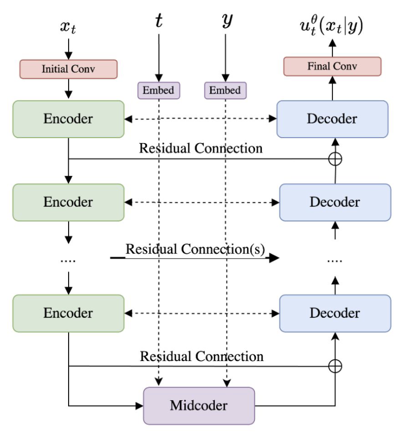
This is a CNN architecture that has encoders that reduce the number of pixels while increasing the number of channels. The decoder layers reverse this process. The encoder and decoder blocks each have two “residual layers”. The midcoder is just a sequence of 3 residual layers.

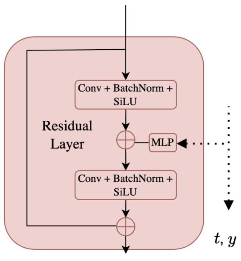
The time and condition are mapped to embeddings. All of the residual layers have access to these embeddings. They are processed through an MLP to map these embeddings from the initial embedding dimension to the number of channel at this block. The embeddings are then added to every pixel.

Diffusion Transformers

The time and condition are just added as tokens to the input, but at every block.

Generative modeling can also be applied in the latent space. The idea here is that images contain a lot of high frequency details that the model doesn’t need to worry about. There are encoders and decoders that map images to a latent space. The conditioning is only applied to the Denoising U-Net which generates images in the latent space. This means that the sampling can also be done in lower dimensions and then mapped back to the pixel space at the end.

Stable Diffusion 3 uses a pretrained autoencoder and conditions on text embeddings for text conditioning.

Resources

• https://diffusionflow.github.io/
• https://arxiv.org/pdf/2406.08929